Final publication date 14 Jun 2023
A Study on the Machine Learning-Based Apartment Price Index
 ; Kim, Kyung-Min***
Abstract
The house price index is essential for assessing the housing market conditions and predicting future changes in the market. However, the two main methods for calculating the housing price index, the appraisal-based index and transaction-based index, have significant drawbacks. The appraisal-based index method has issues such as smoothing and lag bias owing to the involvement of human appraisers, and it also requires significant manpower for calculations. The transaction-based index method requires numerous transaction samples to achieve statistical significance, making it challenging to be created for small regions or when transactions are scarce. To address these issues, we propose an alternative approach that employs a machine learning model to estimate time-series transaction prices for individual apartments and builds a Laspeyres index with the estimated prices. We demonstrated the model’s ability to capture serial correlation of house prices, enabling accurate estimations even with unobserved potential prices. Comparing our prediction-based index to existing Korean house price indices, we observed local smoothing but overall alignment with the global trend of the transaction-based index, facilitating smooth index calculation for small areas. This study offers a novel method for house price index calculation that mitigates limitations of traditional approaches by using machine learning for more precise house price estimation, even with limited housing transaction data.
Keywords:
House Price Index, Machine Learning, Artificial Neural Network, House Price Valuation, Smoothing키워드:
주택가격지수, 머신러닝, 인공신경망, 주택가격산정, 평활화Ⅰ. Introduction
The house price index plays a crucial role in various analyses concerning the housing market. These analyses are used to confirm current house price levels, evaluate the impact of government agencies' real estate policies, and predict market prospects. Consequently, several methodologies have been introduced to create a house price index that captures real market trends with high precision, allowing for more accurate analyses.
Price indices in fields other than real estate, such as stock market indices and consumer price indices (CPIs), often use the method of weighted averaging of price levels of products in the market at every point in terms of the shares of relevant products in the entire market. Specifically, in the stock market, many indices use the market capitalization method, where trends in individual stock transaction prices are weighted by the number of listed stocks. Although there are variations in specific calculations, generally, indices are generated by dividing the current market capitalization by market capitalization at a reference point and then multiplying the result by the reference point index. However, changes in the market such as the listing of new stocks can lead to disruptions in continuity due to not only natural fluctuations in market prices but also external factors. In such cases, a method of adjusting existing market capitalization is adopted to ensure continuity. As for indices using the market capitalization method, representative ones are the Korea Composite Stock Price Index (KOSPI) and the Korean Securities Dealers Automated Quotations (KOSDAQ) Index in South Korea, and the Standard and Poor’s 500 (S & P 500) and the Nasdaq Composite in the United States.
In the case of South Korea, research on price indices using transaction data from the real estate market has been conducted because all house transaction prices are recorded and disclosed. However, to date, indices based on real transaction prices have not adopted a market capitalization method like that used in stock indices. Previous studies have argued that transaction price information at every point in time is required to create a market capitalization index; however, unlike other markets, it is difficult to apply a market capitalization index to the housing market because housing is not traded at every point in time (Lee, 2007; Park, 2009; and Jung et al., 2014).
Strictly speaking, stocks are not transacted repeatedly at individual points, either. However, due to repeated transactions of identical stocks generally occurring at very short intervals (units of seconds), it is possible to capture transaction prices at almost every point within hours or days. Additionally, the method of extending immediately preceding transaction prices can be used for points where transactions did not occur.1) On the contrary, due to the characteristics of individual houses being heterogeneous and the housing market having longer market cycles, the housing market may not witness repeated transactions of the same house for several months or even years. Consequently, at points where transactions did not occur so that prices cannot be captured, simply extending immediately preceding transaction prices, as is done with stocks, can lead to a greater disparity from potential prices that would have formed if actual transactions had taken place.
For these reasons, various methods are utilized to capture sequential changes in transaction prices while controlling the heterogeneity of houses. These methods include statistical approaches such as the repeat sales model or the hedonic price model as well as the use of the market capitalization method with the direct human appraisal of individual house prices at each point in time. However, in the former case, it is difficult to produce a price index for small areas because many transaction samples are necessary to secure statistical significance. Even when considering larger geographic scopes, the index can become unstable during periods of insufficient transactions. On the other hand, in the latter case, the problem lies in the inability to produce an index based on the prices of all houses, as it necessitates a large workforce for the task of price calculations. Instead, the index should only reflect price fluctuations of sample houses under evaluation. Moreover, concerns have been raised about potential biases resulting from humans' direct calculations of prices (Geltner, 1991; and Eriksen et al., 2019).
To supplement the limitations of existing price index methodologies, this study proposes a price index based on the market capitalization method that utilizes the artificial neural network (ANN) model, a type of machine learning (ML) technique, to estimate the prices of all houses at each point; model is based on such estimated prices. Important features of ML techniques that distinguish them from traditional statistical methods are pattern recognition (PR) and self-learning. This means that the ML model can capture complex and non-linear relationships on its own, without researchers having to establish them (LeCun et al., 2015). Consequently, unlike the use only of variables having linear relations such as house areas or depreciation in the traditional hedonic price model to explain house prices, when ML techniques are used, prices can be estimated even based on information not having linear relationships such as geographic coordinates (Kim and Kim, 2022). Earlier research has shown that levels of accuracy equal to appraisers’ direct estimations of prices can be reached through the ML model (Bae and Yu, 2018a).
Based on discoveries from previous research, this study aims to demonstrate that the ML model, by learning information on transaction points in apartment transactions, can effectively capture the serial dimension of apartment transaction prices. Consequently, the model can more accurately estimate potential prices for points without transactions compared to the simple extension of immediately preceding transaction prices. The main objective of this study is to introduce a house price index methodology based on ML modeling that overcomes the limitations of existing transaction-based indices and appraisal-based indices alike.
The study's structure is as follows. Chapter II provides a review of the theoretical background of the house price index and recent research using ML. Additionally, it highlights the distinctive features of this study. Chapter III formulates specific research hypotheses and outlines the scope of the study, drawing insights from previous research findings. Chapter IV introduces the expressions for the ANN model, serial autocorrelation tests, and market capitalization index method, all of which are utilized as analysis methodologies in this study. Chapter V offers a comprehensive description of the data used for the model's learning process along with presenting basic statistics. Also, this chapter outlines the ANN model's hyperparameters. In Chapter VI, the results of both the model's learning process and the construction of the house price index are presented. Finally, Chapter VII summarizes the study's findings and discusses their implications. It also addresses the limitations of this study and future research tasks.
Ⅱ. Literature Review
1. Research on House Price Indices
House price indices can broadly be classified into transaction-based indices and appraisal-based indices (Lee and Lee, 2008; Park, 2009; and Geltner, 2011). According to Geltner (2011), transaction-based indices can further be classified into methods that use statistical models and those that simply sum up the average or median values of transaction prices at every point. Indices based on average or median values have the advantage of not requiring analysts’ statistical knowledge and computing performance. However, they cannot facilitate comparisons among points due to the uncontrolled heterogeneity of houses transacted at each point. Statistical models are used to control houses’ heterogeneity, and two representative types are the repeat sales index and the hedonic price index. The repeat sales index controls the heterogeneity of houses through the method of producing an index by using trading pairs of identical houses that have been transacted at least twice. In this approach, it is assumed that changes in the quality of houses do not occur over time (Barr et al., 2017). The hedonic price index relies on the hedonic price model, where the sales prices of houses are the dependent variable, while various characteristics of houses serve as explanatory variables. By incorporating houses' characteristics as explanatory variables in the model, the cross-sectional fluctuations of house prices can be controlled. Transaction point information is entered in the model as a dummy variable, then serial fluctuations in house prices are captured based on the regression coefficient of transaction point dummy variables (Geltner, 2011). Additionally, with the hedonic price index, there is also the time-varying parameter model, where a model consisting of identical combinations of characteristic variables at each point is estimated, and identical characteristic values are entered in each cross-section model to estimate houses’ potential prices, thus calculating the index (Lee, 2007).
One major drawback of the transaction-based index is the requirement to secure enough transactions. Park (2007) demonstrated this issue through simulations in a market with low transaction frequency, where a hedonic price index was generated. The results showed that when transaction samples were inadequate, the volatility of the index increased, and the influence of outliers became significant. Consequently, when small areas such as towns (eup), townships (myeon), and neighborhoods (dong) or station areas are considered as the spatial scope of index production or when transactions decrease during real estate downturns, there is a possibility of encountering substantial noise and producing an unstable index due to the failure to obtain sufficient transactions. In relation to this, there has been an increase in the demand for subdivided indices at the level of small areas, driven by issues such as neighborhood-specific real estate policies. Song et al. (2020) have also argued that, to counter the instability of the index, corrective methods such as moving averages or sample overlaps should be employed.
Next, the appraisal-based index constitutes a method in which individual house prices are regularly appraised, and the price index is calculated through the flow of housing market capitalization produced with the appraisal price per house as the basic price. According to Suh (2009), in South Korea, KB Kookmin Bank (hereafter “KB”) and Real Estate 114 (R114) have produced price indices based on appraisal prices. R114 has investigated the upper and lower limit prices per apartment complex and per area through real estate agents. Similarly, KB has utilized the method of investigating market prices for every point based on transaction prices in cases where transactions occurred. When there are no transactions, they rely on cases of nearby transactions collected by real estate agents in relevant areas. As of April 2022, a total of 36,300 sample houses nationwide were being tracked.
With the appraisal-based method, under the premise that there exist accurate appraisal prices at each point, the price index can be produced in a comparatively intuitive manner. Unlike the transaction-based index, a stable index flow can be constructed even when the number of transaction samples is insufficient. However, the following drawbacks have been pointed out. First, the scope of price index production is limited to certain groups of houses that are regularly appraised (Hill and Steurer, 2017). This is because a vast number of appraisers is necessary in order to appraise potential prices at points where transactions have not occurred for the total houses. As a result, fluctuations in the prices of houses other than sample houses are not adequately reflected in the index. The second issue that has been identified is the phenomenon of smoothing. This arises from the conservative approach taken by human appraisers when evaluating individual houses. They tend to base their assessments on past appraisal cases of the same houses, leading to a tendency to make cautious adjustments. Geltner (1991) has explained this phenomenon with the following “partial adjustments model”:
| (1) |
 is the true appraisal price of house i at point t, and
 is the purely random appraisal error. However,
 , the final appraisal price of house i at point t, is influenced by
 , the final appraisal price at the immediately preceding point, and the degree of such influence changes according to αi, which signifies “confidence” regarding the house’s appraisal price at the immediately preceding point i. The parameter αi has a value ranging from 0 to 1. When α αi is 1, then the immediately preceding appraisal price is disregarded. On the contrary, when αi is 0, then appraisal is not performed at the current point, and the immediately preceding appraisal price is extended without any adjustment. Geltner (1991) has argued that, no matter how accurate individual house price appraisals are, unless prices are completely recalculated at every point, smoothing will persist in the index consisting of appraised houses. Lee and Lee (2008) have supported this notion, revealing that αi is measured to be 0.35 or 0.48 in KB’s appraisal-based house price index, which demonstrates the existence of the smoothing phenomenon. This smoothing presents advantages such as reduced sensitivity to outliers in house transactions and the potential for decreased noise in the price index. However, there are drawbacks associated with this approach. One such drawback is the difficulty in capturing turning points in the housing market and using this index as a basis for timely policy establishment. This is due to their inherent lag, exhibiting a time delay of approximately 1-2 quarters compared to the current market situation (Lee and Lee, 2008; Hill and Steurer, 2017; and Song et al., 2020). In addition, Eriksen et al. (2019) have also pointed out the possible existence of the problem of a conflict of interest. This occurs when certified public appraisers, in the process of carrying out their duties, may introduce biases in house price appraisals due to influence from interested parties such as licensed real estate agents in the areas.
2. Research on ML-based Price Indices
In recent years, there have been attempts to construct price indices through ML techniques, which exhibit higher accuracy than traditional statistical models, to overcome the limitations of existing house price indices. Barr et al. (2017) created a house price index for Los Angeles during 2000-2016 at the individual ZIP code level. To achieve this, a cross-section regression model where house transaction prices were calculated per quarter was constructed through the gradient boosting method, an ML technique. For comparison purposes, the median transaction price index and the repeat sales index were also calculated under identical conditions. Pairs of repeated transactions of identical houses were extracted from a randomly separated test set, and price increase rates predicted for respective trading pairs through actual price increase rates and index were contrasted to evaluate the accuracy of the index. The analyses revealed that noise was less, and accuracy was higher in the ML-based price index than in median prices and the repeat sales index. However, the price index in this research was generated solely for individual ZIP codes and did not extend to create a price index for the entire area.
Bae and Yu (2018b), using the random forests and the ANN models, both ML techniques, calculated individual apartment prices per point using the Gangnam-gu district in Seoul as their focus. They then computed the geometric mean of the increase rates in comparison to the reference point for each sample, resulting in the generation of a price index for each point. Here, data on transaction prices per point and per sample house in the past n months were used to construct a cross-section regression model, and the numbers of months were designated as 1 month, 3 months, 6 months, and 12 months, respectively, in conducting tests. According to the analysis results, volatility was larger when the learning data covered shorter periods. Conversely, when the period was longer, volatility decreased, resulting in higher stability. However, it became more challenging to reflect the latest trends, and the index tended to exhibit smoothing. In addition, when the house price trend index announced by the Korea Real Estate Board (REB), the REB’s transaction-based price index, and the ML-based index were compared, they found that the ML-based index exhibited greater volatility than the existing indices. Consequently, it was pointed out that there was a need to supplement sample prices with qualitative analysis conducted by researchers.
Kim et al. (2022) constructed a model explaining apartment prices in 25 autonomous districts in Seoul through ANN and random forests. Through their analyses, they found error rates to be the lowest for the random forest model and produced a price index based on the trained random forest model. This research performed modeling through the method of entering region and time dummies along with apartment characteristic variables in the model. A price index was then produced by adjusting the values of the region and time dummies while fixing characteristic variables using average values. The results showed that the index derived from this research, which performed modeling based on transaction prices, exhibited a greater range of fluctuations compared to the existing KB and REB house price indices.
3. Chapter Summary
Previous research on house price indices can be largely classified into transaction-based indices, which perform statistical modeling based on transaction samples, and appraisal-based indices, in which price indices are generated in a manner similar to composite stock market indices, assuming the existence of a directly appraised price flow for each point and individual house. However, each type of indices has its own strengths and weaknesses. Transaction-based indices can provide a more accurate representation of the market situation, but their effectiveness relies on the number of transaction samples or house transactions, which affects the statistical significance of index values. Consequently, it is difficult to produce stable indices for recessions when transactions drop and for small areas, thus leading to the generation of index flow noise that is not related to actual price fluctuations. In contrast, appraisal-based indices are less sensitive to the number of transactions but require humans’ direct appraisals. This makes it difficult to produce such an index for all houses, introduces smoothing effects, and can give rise to the problem of conflict of interests.
To overcome the limitations of previous research, this study aims to develop a house price valuation model using ML and, subsequently, construct a price index. By doing so, this study intends to address issues that arise from human involvement in price appraisals and resolve the problem of instability, which is a drawback of transaction-based indices. In recent times, there has been increasing research focusing on building more sophisticated house price indices using ML techniques compared to existing methodologies. However, existing research has focused on calculating transaction prices per point using cross-section models that do not incorporate serial information (Barr et al., 2017; Bae and Yu, 2018b). Alternatively, some studies have included serial information in the model such as time dummy variables but have primarily emphasized the overall model's predictive accuracy rather than exploring how relevant variables explain house prices in a serial manner (Kim et al., 2022). Because a price index represents the serial flow of prices, constructing a model that explains the fundamental prices of the index requires an examination of both longitudinal modeling and its impact. Consequently, this study seeks to construct an estimation model through apartment price explanatory variables including time information, to review the model’s accuracy in predictions, and to show that the model can model the serial dimension of house prices. Through this analysis, this study will discuss the distinctive characteristics of the proposed price index.
Ⅲ. Hypothesis and Scope of Study
Based on the findings of earlier research, this study aims to demonstrate the following specific hypotheses.
First, the ANN model can appropriately capture the temporal dimension of prices through information on transaction time. To prove this, the training progress of the ANN model with transaction time information added will be compared to the model without such information, confirming that the inclusion of transaction time significantly lowers prediction errors.
Second, in the prediction errors of a model that effectively captures the temporal dimension of prices, serial autocorrelation will decrease significantly in comparison with the actual transaction price flow. The immediately preceding transaction prices of identical houses can serve as market prices that have a significant impact on subsequent transaction prices. Thus, this study assumes transaction prices as time series with first-order autocorrelation. If a price time series predicted through the modeling process accurately follows the overall price flow, excluding noise, then model prediction errors will primarily consist of uncorrelated noise. Based on this, the degree of serial autocorrelation for transaction prices and prediction error time series will be compared. A significant decrease in autocorrelation within prediction errors will demonstrate that the model effectively captures the temporal dimension of transaction prices.
Third, the model’s predicted price flows will provide more accurate estimates of potential prices at points without transactions compared to the simple extension of transaction prices. Here, the simple extension of transaction prices changes only when actual transactions occur and appears as a straight line when there are no transactions over an extended period. During recessions or periods of reduced transactions, the disparity between potential prices that could have been observed with actual transactions and the recorded transaction price flow can widen. However, if model-produced prices estimate the price flow well, they will be capable of approximating value fluctuations for each point regardless of the presence or absence of actual transactions. Consequently, these estimates will be closer to potential prices. However, since potential prices cannot be directly observed, this study will employ the following method. First, the total transaction data will be randomly divided into training data and testing data. The model will be established with training data, and testing data will be treated as unobserved potential prices. Through this approach, it will be demonstrated that estimated prices at every point, produced by the model, predict potential prices in the separated testing data more accurately compared to simply extending transaction prices in the training data.
Based on modeling results, a market capitalization-based index will be constructed. The index will consist of predicted prices produced by the ML model at every point, weighted by the number of households. The scope of this study will include comparing the index with those from other agencies and interpreting their characteristics.
Ⅳ. Research Methods
To verify the hypotheses above, the following research methods will be employed. First, an ANN model estimating transaction prices will be constructed. This model will be used to calculate individual apartments' prices at each point, and the performance of modeling the serial flow through transaction time information will be assessed. Subsequently, with the price flow estimated on the level of individual apartments as the basic price, an apartment price index based on the market capitalization method will be constructed, and it will be compared with existing publicly disclosed indices.
1. Artificial Neural Networks (ANNs)
ANNs are a type of ML technique with various structures designed to suit different research objectives such as recurrent neural networks (RNNs) and convolutional neural networks (CNNs). This study uses the basic multilayer perceptron structure. The model consists of the input layer, hidden layer, and output layer. Data entered in the network are multiplied by the weights of each layer and then transmitted to the next layer through the non-linear activation function. The model calculates losses by comparing the produced values in the final output layer with transaction prices. The model’s weights are updated in a way that minimizes total losses during training, allowing the model to abstract and learn non-linear relationships among the variables. Here, a model with two or more hidden layers is separately classified as a deep neural network (DNN), and the process of training such a DNN is referred to as "deep learning." Since the 2010s, advancements in computing power and model learning techniques have made deep learning possible and led to its widespread adoption. Deep learning has been demonstrated to outperform traditional linear regression models in terms of prediction performance (Chollet, 2017; and Loo, 2019).
Two main drawbacks of ML techniques that have been pointed out are that they are black box models and can be easily overfitted. Unlike traditional statistical models where relationships among variables can be expressed and interpreted as regression coefficients, neural networks in black box models consist of numerous weights so that it is difficult to express relationships among variables with a single slope value. Thus, this study aims to demonstrate the model's ability to capture the temporal aspect of prices by analyzing the patterns of model prediction errors. Overfitting refers to a phenomenon where the model is overly optimized to the training data, leading to a decline in its ability to make accurate predictions on new, unseen data. To prevent overfitting, a portion of a training data set (henceforth referred to as the “training set”) is separated as a validation data set (henceforth referred to as the “validation set”). Prediction errors are then evaluated using both the training set and the validation set during the model's learning process. The weights are adjusted until errors in the validation set are minimized, establishing the model's final configuration. Subsequently, if prediction errors on the test data set (henceforth referred to as the “test set”) are similar to validation set-based prediction errors, then overfitting is considered to be absent, and the model will be finalized.
2. Serial Autocorrelation Testing Methodology
To demonstrate that the model can effectively capture the temporal dimension of transaction prices, this study aims to compare the serial autocorrelation of transaction prices and prediction errors for individual houses in the test set. It can be simply expressed as follows:
| (2) |
Here, t is the time period, yt is the transaction price, Xt is the explanatory variable including the transaction time, ϵt is the model prediction error, ρ is the first-order autocorrelation coefficient, and et is simple white noise that does not include autocorrelation. If ρ0, which is the autocorrelation coefficient of the price time series, exhibits a significant positive value, but ρ1, which is the autocorrelation coefficient of the prediction error time series, is either 0 or significantly smaller than ρ0, then the model can be considered to explain effectively the autocorrelation of transaction prices.
However, with transaction information from multiple houses, the unique non-serial characteristics of individual houses can act as fixed effects, causing individual effects unrelated to the time series to persist in the model's prediction errors. This can be expressed as follows:
| (3) |
i represents an individual house, yi,t is the transaction price of each house at each point, Xi,t is the explanatory variable fluctuating serially, Zi is the fixed explanatory variable not changing serially, μi is the unexplained fixed effects of individual houses, and ϵi,t is individual and serial residuals. To test serial autocorrelation in such panel data, the first-difference method proposed by Wooldridge (2002) and Drukker (2003) can be applied. When the above expression is first-differentiated, it is as follows:
| (4) |
When the expression is differentiated in this manner, fixed effects are eliminated, leaving only serial explanatory variables and residuals. According to Wooldridge (2002), the correlation coefficient of the differentiated time series and first-order lag time series of residuals, denoted as Corr Corr(Δϵi,t, Δϵi,t-1), becomes -0.5 when ϵi,t does not have serial autocorrelation. Based on this, Drukker (2003) has demonstrated that it is possible to test the panel data’s serial autocorrelation by regressing the difference time series of model residuals on the first-order lags and examining whether the coefficient value is -0.5.
Consequently, this study aims to confirm whether the ML model has appropriately performed serial modeling by obtaining the first-order autocorrelation coefficient of transaction prices and prediction errors while simultaneously conducting tests based on Wooldridge’s and Drukker’s method to eliminate individual houses' fixed effects.
3. Price Index Methodology
In this study, the transaction prices of individual houses at each point are predicted through a model that has learned serial information on house prices, and the number of households is weighted to calculate market capitalization, based on which a price index is constructed. The logic behind the price index is an application of the method used for the S & P 500 index, which has been made publicly available by S & P Dow Jones Indices, LLC. The price index is based on the Laspeyres method but has been modified to ensure that any change to stocks constituting the index at individual points results in the revision of standard market capitalization. This modification prevents any disruption in the temporal continuity of the index. The specific expressions are as follows.
First, the basic formula of the Laspeyres index, where the index value at the reference point is established as 100, is expressed as follows:
| (5) |
I is the index, P is the price, Q is the number of households, i is an individual house, 0 is the reference period, and t is the point at which the index is calculated. While this expression assumes no change to the index’s constituent stocks, the total number of houses can vary due to factors such as new constructions or demolitions. This can disrupt the continuity of the index flow when calculating the simple market capitalization ratio. When the index is devised only based on houses that exist throughout the total time series to prevent such disruption, the prices of newly constructed and demolished houses are not reflected in the index. To address this issue, the basic Laspeyres index is modified as follows. First, market capitalization at every point is established as the numerator, and the divisor that can fluctuate at every point is established as the denominator:
| (6) |
Dt is the divisor at point t. Because Qi,t is not fixed at the reference point in the modified index, market capitalization at every point in the area becomes the numerator. The divisor is adjusted each time there is a newly constructed house or a demolished house, thus allowing the index to continue without the index value being affected by changes to market capitalization caused by changes to the total amount. When the completion of the construction of a new house at point t is presumed, it is as follows:
| (7) |
Here, s represents the house newly constructed at point t and is separate from i, which is a set of houses that existed at point t-1 as well. If the divisor is not changed, fluctuations in market capitalization because of the presence of a newly constructed house can cause the index to rise considerably. Therefore, the divisor is adjusted so that constituent items up to point t-1, the index produced through the divisor at point t-1, and the index produced including newly incorporated items will be identical. When expressed as an expression, it is as follows:
| (8) |
Dt, the divisor adjusted at point t, is not actually used in calculations of the index at point t but is used from point t+1 onward. Therefore, if a new house is incorporated at point t, first, It, which is the index at point t, is calculated through the divisor and constituent items up to point t-1, disregarding the new house. Next, the divisor is adjusted by dividing market capitalization at point t, recalculated after incorporating the new house, by It. Subsequently, when there are no changes to houses’ constituent items from point t + 1 onward, the divisor newly adjusted at point t is used in this method.
In cases in which a house is excluded due to its demolition, the order of adjusting the divisor is inverted and correction is performed so that the index produced through houses remaining even after point t and the price index produced including houses excluded from point t onward will be identical. When a house demolished at point t is established as r, this is expressed as an expression as follows:
| (9) |
Consequently, when cases of the coexistence of newly constructed and demolished houses at each point are hypothesized and generalized, the two expressions can be combined and expressed as follows:
| (10) |
Ⅴ. Description of Data and Model
1. Data
The focus of object analysis in this study was limited to apartments because apartments are relatively standardized assets in South Korea, and transactions of identical apartments are more frequent than those of detached houses, making it easier to create the price index (Jeong, 2014; and Kim et al., 2015). The source of transaction prices for the model’s learning process was the apartment sales data provided by the Ministry of Land, Infrastructure and Transport (MOLIT) of South Korea. The data covered cases of transactions in Seoul from January 2006 to December 2022, and, after excluding canceled transactions, a total of 1,184,083 cases of transactions were used. Furthermore, to control characteristics specific to each apartment area, data from the apartment complex database provided by the South Korean prop-tech company Zigbang was used. Additionally, to calculate market capitalization, which forms the basis of the price index, information from Zigbang on the number of households per apartment complex area was utilized.
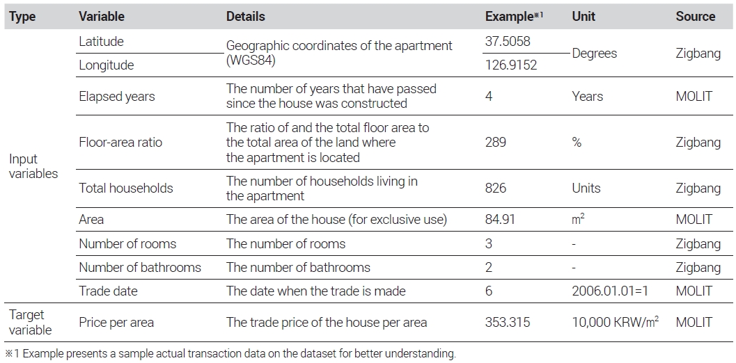
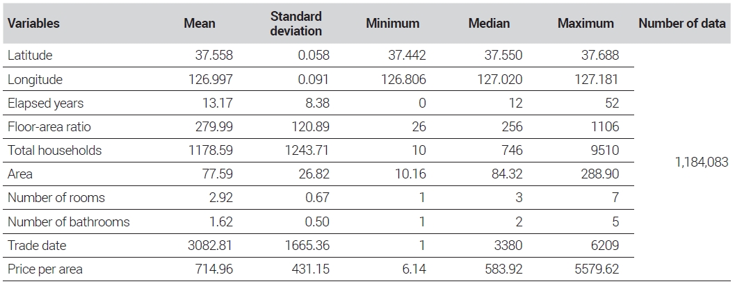
The model’s explanatory variables included the longitude and latitude coordinates of each apartment complex, the number of years since construction completion, the floor-area ratios, the total number of households per apartment complex, the apartment areas, the numbers of rooms, the numbers of bathrooms, and the transaction dates. The dependent variable was the sales price per area. Specifically, the longitude and latitude coordinates, the number of years since construction completion, the floor-area ratios, and the total number of households were determined for each apartment complex. The areas, the numbers of rooms, and the numbers of bathrooms were determined based on the area of each house in an apartment complex. Additionally, for the transaction date variable, January 1, 2006, when apartment transactions were first disclosed, was set as day 1, and this number was incremented by 1 for each subsequent day. Although this study’s price index was calculated every month, transaction date information was entered daily because, in the case of large apartment complexes with frequent transactions, price fluctuations can occur even at intervals shorter than a month. Furthermore, unlike earlier research based on the hedonic price model, variables such as administrative division dummies or season dummies were not included. Instead, spatiotemporal characteristics were explained through the geographic coordinate and transaction date variables. This decision was made due to the overfitting phenomenon that occurred when dummy variables were included in the model, exceeding the permissible level. Tables 1 and 2 provide a summary and descriptive statistics of the data sets, respectively.

Summary of dataset
Descriptive statistics
2. Model Configuration
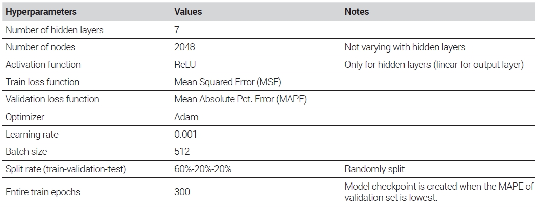
This study utilized Python’s neural networks library Keras (ver. 2.4.0) and employed Scikit-Learn's StandardScaler function to standardize the input variables, thereby enhancing learning efficiency (Chollet, 2017). To find the optimal neural network model, it is necessary to explore various hyperparameter combinations including the model's structure, number of training epochs, and loss functions. As there is no predetermined rule, multiple combinations need to be tested repeatedly (Lenk et al., 1997). Through literature review and repeated learning and searches, this study obtained the optimal hyperparameter combinations, which are summarized in Table 3. To prevent the model from being overfitted to the training data, the data set was randomly divided into the training set, validation set, and test set. During the training process of a total of 300 epochs, the model at the point where errors in the validation set were minimized was selected as the final model. Additionally, the separated test set was used to confirm the error rates of the final model.
Summary of Neural Network Hyperparameters
VI. Results
1. Model Training
Figures 1 and 2 display the learning progress in the full model and the reduced model, respectively, without the transaction date variable. After 300 epochs of learning, the mean absolute percentage error (MAPE) value for the validation set, which was separated from the training set, converged to around 5% in the full model that included transaction dates as an input variable. However, in the case of the reduced model, the MAPE value for the validation set remained above 6%, failing to reach the same level as the full model.

Training progress of full model

Training progress of reduced model without trade date variable
Meanwhile, when the graph of learning progress in the full model in Figure 1 is examined, the training set-based MAPE value continuously dropped to around 4.2%, whereas the validation set-based MAPE value tended to converge at approximately 5.1%, failing to fall below this threshold. This indicates a potential overfitting of the model to the training set. Consequently, the 299th epoch, where the validation set-based MAPE value was minimized to 5.115%, was chosen as the point for establishing the final model. To assess the model's accuracy further, the test set, distinct from both the training set and the validation set, was utilized. The MAPE value from the test set amounted to 4.98%, lower than the validation set-based MAPE value, indicating that the general prediction performance of the model for new and unseen data was acceptable. Moreover, for the model in which information on transaction dates was not included, the test set-based MAPE value was also measured through the model at the epoch minimizing the validation set-based MAPE value, and the result was 6.49%. To determine the statistical significance of the difference between the two MAPE values, paired sample t-tests were conducted on the average difference between absolute percentage errors produced from the models. The t-value was 129.967, and the p-value was 0.000, confirming that the decrease in the model error rate through the usage of the transaction date variable was statistically significant.
2. Serial Autocorrelation Test
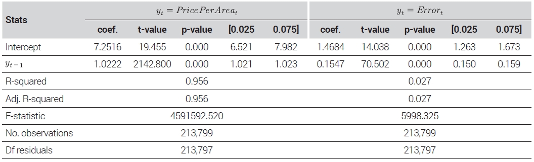
To prove the research hypothesis that if the model effectively captured the temporal dimension of apartment transaction prices, serial autocorrelation would decrease considerably in model prediction errors in comparison with the transaction price flow, serial autocorrelation of prices and prediction errors in the test set was confirmed. As the test set encompasses diverse apartments, housing units of the same areas in individual apartment complexes were considered identical houses, and each transaction in the test set was matched with immediately preceding transactions of the same house.2) The total number of test set transactions amounted to 236,817 cases. However, the first-point transactions of individual houses were excluded from the analyses due to the unavailability of immediately preceding transaction prices. Consequently, matched transaction data on 213,799 cases were analyzed. The regression results for the price per area and prediction errors of each sale in terms of the immediately preceding cases are presented in Table 4. According to the results of the analyses, for price per area time series, the first-order autocorrelation coefficient and the R-squared value were high, amounting to 1.0222 and 0.956, respectively. This indicates a strong linear correlation between transaction price time series and the immediately preceding prices of identical houses. However, in the case of the model’s prediction error time series, the first-order autocorrelation coefficient was 0.1547, and the R-squared value was 0.023, respectively. If temporal modeling were not performed at all, model prediction errors would exhibit serial correlation with immediately preceding transactions, as with transaction price time series. In such a case, it would be possible to obtain both a high R-squared value and an autocorrelation coefficient approximating 1.0. However, the results show that, through the model, the temporal dimension of transaction prices was effectively modeled. In addition, the non-zero regression coefficient value of prediction errors further confirmed that the model significantly explained the temporal dimension but could not completely explain it.
Regression result: test-set price per area and prediction error to their time lags
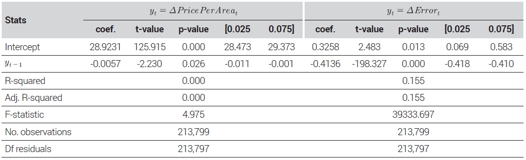
Meanwhile, because the test set in this study includes diverse apartments, individual apartments’ fixed effects may have influenced the results. To verify serial autocorrelation after eliminating fixed effects from these panel data, the Wooldridge-Drukker test method was applied. For both transaction price and prediction error time series, differences from immediately preceding transactions of the same houses were calculated to remove fixed effects, and relevant difference time series were regressed to immediately preceding transactions. The results are recorded in Table 5. According to Wooldridge (2002), the regression coefficient approaches 0 when strong serial autocorrelation exists, indicating a random walk pattern. In contrast, the coefficient approaches -0.5 when there is no autocorrelation, representing white noise time series. According to the results, the regression coefficient for price per area approximated 0, indicating the presence of strong autocorrelation. For the prediction error time series, the regression coefficient was -0.4136. While this explained serial correlation in terms of the model considerably, the regression coefficient of prediction errors significantly fell short of -0.5, indicating that some degree of serial correlation remained. This result of the Wooldridge-Drukker method-based test is consistent with the analyses of the original time series.
Regression result: test-set price per area and prediction error to their time lags (1st-difference)
3. Evaluation of Potential Price Prediction
Figure 3 compares between “actual transaction prices” recorded in the training set and “predicted values” generated by the trained ANN model for an 84.9 m2 Ricenz Apartment in Jamsil-dong, Songpa-gu, Seoul from 2011 to December 2022. The solid line represents the transaction price flow recorded in the training set, with the immediately preceding prices extended for points without transactions. The dotted line represents model prediction prices at every point, and the graph confirms that model prediction prices fluctuate even at points when transactions have not occurred. The round dots represent the transaction prices included in the test set. The data in the test set have not been used in training the model. Thus, this study considers them as “unobserved potential prices.”

Model-predicted, actual, and potential price: Jamsil Ricenz Apartment 84.9 m2
To prove the hypothesis that temporal price modeling improved potential price predictions for points without transactions, this study compared the error rates of the transaction price flow per apartment complex area3) in the training set with the predicted price flow produced by the model trained on potential prices. The analysis included 231,998 cases out of a total of 236,817 cases in the test set, excluding 4,819 cases that did not have the immediately preceding transaction prices of identical houses in the training set. According to the results, the difference between the potential prices of the test set and the actual transaction price flow had a MAPE value of 6.24%, while the difference between the same potential prices and the model's predicted prices had a MAPE value of 4.90%, resulting in an error rate reduction of approximately 1.34%p through ML modeling. This shows that, in comparison with the simple extension of immediately preceding transaction prices, estimated prices through modeling resulted in a decrease in the error rate by approximately 1.34%p. To confirm the statistical significance of this difference, a paired sample t-test was performed, yielding a t-value of 104.137 and a p-value of 0.000, indicating that the decrease in the error rate because of the model was statistically significant. Consequently, it can be confirmed that the flow of the model's estimated prices is closer to unobserved potential prices than the flow of simple real transactions, which are noisy and may not capture changes in value when there is no transaction.
4. Price Index Based on Model-Estimated Prices
Price trends for individual apartment complexes’ area types were estimated using the trained model. The estimated price per area was then multiplied by the area to calculate estimated prices for each point. Trends in apartments’ market capitalization, obtained by weighting estimated sales prices with the numbers of households in areas per apartment complex, were aggregated to produce the monthly price index. The reference point of monthly price estimations was the first of each month, and the prices for January 2006-December 2022 were estimated. When there were newly constructed and/or demolished houses, the divisor was modified to ensure index continuity, following the method presented in Chapter III. The total number of apartment complexes in Seoul included in the calculation was 7,463, and the number of area types amounted to a total of 46,024.
In Figure 4, the ANN model’s estimated price-based price index (henceforth referred to as the “model-estimated price index”), KB’s house price trend index, the REB’s house price trend index, and the REB’s transaction-based price index for all apartments in Seoul have been reconverted so that the figure for January 2017 would be 100 and are compared.

House price index comparison (Seoul, apartment sales, 2017.01=100)
In the overall serial trends, the model-estimated price index exhibited trends most similar to those in the REB’s transaction-based price index. The REB’s house price trend index showed the lowest overall price volatility, and KB’s house price trend index exhibited trends in between. This was presumably because while KB’s and the REB’s house price trends reflected in the indices not only transactions but also bids regarding sample houses, the model-estimated price index and the REB’s transaction-based price index were based on identical data sets, only using transactions of the total houses.
In detail, through index movements during major recessions in 2008, 2018, and 2022, it can be confirmed that the REB’s transaction-based price index is more sensitive than the model-estimated price index. The model-estimated price index captured only fluctuations on a level similar to those of KB’s and the REB’s house price trend indices, thus confirming the existence of smoothing of the index. This tendency, in relation to analysis results showing the partial existence of autocorrelation with identical houses’ immediately preceding transaction prices in the model’s predictions of serial transaction prices earlier, is interpreted as being because of the existence of the conservative price appraisal tendency explained by Geltner’s (1991) partial adjustments model also in model-estimated prices.
Meanwhile, the model-estimated price index is produced by aggregating the price flow on the level of individual apartment areas. As for the flow of basic prices, there is a tendency for transactions to fluctuate more gently than such a flow, as illustrated in the example in Figure 3. Consequently, the model-estimated price index can be produced stably even for small areas with insufficient transaction samples such as towns, townships, and neighborhoods instead of a wide scope such as the entire Seoul. Figure 5 shows the production of the model-estimated price index for 14 legal neighborhoods in Gangnam-gu, Seoul as an example. The diagram confirms that, even for the scope of small areas, it is possible to suppress noise and create a smooth price index flow.

Model prediction-based index: Dong-level, Gangnam-gu, Seoul (2017.01=100)4)
VII. Conclusion
To address the limitations of existing house price indices, this study proposed using ML techniques to estimate the serial house price flow and develop an apartment price index. Among the current house price index methodologies, transaction-based indices such as the repeat sales index and the hedonic price index suffer from producing unstable indices in areas with limited transactions or small sample sizes. On the other hand, the appraisal-based index that relies on appraisers' valuations encounters challenges in appraising all houses at each point due to workforce constraints, leading to the use of only certain sample houses for index production. Additionally, the conservatism of house price valuations can introduce smoothing in the appraisal-based index.
Building on previous research, which demonstrated that ML models could achieve house price valuations comparable to human appraisals, this study developed an apartment price index based on market capitalization. The prices at each point were estimated using a model that underwent learning, considering transaction prices and the characteristics of apartment transactions including transaction dates. Unlike recent research that used ML in a cross-section model to estimate the serial flow of house prices, this study incorporated transaction time information, allowing the model to capture the temporal dimension of apartment prices. The characteristic of the price index constructed was thus interpreted.
A summary of the results based on the research hypothesis is as follows. First, under identical conditions, the ANN model demonstrated higher accuracy in estimating prices when it learned information on transaction time. The inclusion of transaction time information resulted in a test set-based MAPE value of approximately 4.9%, which was statistically significantly lower compared to models without transaction time information. Second, this study demonstrated that the model, which learned information on transaction time through serial autocorrelation tests regarding the test set, explained the serial dimension of prices to a considerable extent. However, it can also be confirmed that the serial correlation of prediction errors has not been fully resolved, partly remaining. Third, in comparison with the actual flow of transaction prices, the model’s estimated prices were able to predict potential prices at points without transactions more accurately and, even for points without actual transactions, gently estimated price fluctuations.
After estimating the prices of individual apartments per month based on the trained model and producing market capitalization by multiplying the estimated prices by the number of households per individual apartment area, the Laspeyres index was calculated. When the price index produced for the entire city of Seoul was compared with external agencies’ indices, the former showed similarities to the REB’s communal housing transaction price index flow in the overall trend and exhibited greater fluctuations compared to KB’s and the REB’s house price trend indices. Unlike KB and REB price trend indices, which are produced only for sample houses instead of all houses, the REB transaction-based price index is a repeat sales index produced based on cases of transactions of total apartments. This similarity presumably originates from the fact that the price index in this study is also produced by the model that has learned to estimate transactions of all apartments as accurately as possible. In contrast, when examining detailed fluctuations, it was evident that there was a greater tendency toward smoothing compared to the REB’s transaction-based price index. This phenomenon could be attributed to the fact that the model in this study could not explain serial autocorrelation completely through information on transaction time. As a result, the predicted prices of the ML model also exhibited a serial smoothing effect as did the appraised prices.
Meanwhile, because the price flow could be smoothly generated at the individual apartments level, it was evident that the price index for small areas such as towns, townships, and neighborhoods, too, could be produced seamlessly. Therefore, the apartment price index developed in this study, based on ML model-estimated prices, can mitigate noise and generate a stable index even for small areas with limited transaction data. This capability makes the price index a valuable supplement to existing ones. In the future, by utilizing this methodology to produce a price index for specific station areas or housing zones, further research can be conducted on topics such as analyzing the effects of small areas’ issues on the house price flow.
The limitations of this study are as follows. First, the method suggested in this study of introducing an ML model, unlike existing appraisal-based indices, makes possible the production of a price index composed of the total number of houses. However, it failed to fully resolve the problem of smoothing, which is a characteristic of appraisal-based indices. Consequently, in comparison with the transaction-based index, the price index in this study may not be as sensitive in capturing temporary impacts on the market. This limitation is likely due to the model's inability to completely explain serial correlation in valuations of individual houses. Therefore, future research should focus on enhancing the model's ability to resolve serial autocorrelation and improve its sensitivity in capturing temporary impacts. Second, this study did not conduct a comprehensive comparison of different index methodologies to determine which one was better. Although the proposed index successfully depicted a stable price flow for small areas, this study lacks objective metrics to assess improvements in index stability compared to other methodologies such as the repeat sales index. Furthermore, there is a lack of in-depth discussion regarding the extent to which noise in small areas should be removed or accounted for. Therefore, future research should focus on conducting thorough comparisons of index methodologies using objective evaluation criteria to assess the stability and accuracy of the index flow in reflecting actual market trends. Third, considering the nature of ANNs that start with random weights and converge on specific values during the learning process, even when models are constructed using identical transaction data and hyperparameters, index values can vary each time they are produced. The fact that already produced index values can be modified in the future due to this randomness raises concerns about the reliability of the index. Therefore, it is necessary to review the volatility of produced index values resulting from the randomness of the model. Addressing this issue is left as a task for future research and will ensure more robust and reliable results.
Acknowledgments
This work was supported by SNU Environmental Planning Institute.
Notes
References
-
Bae, S.W. and Yu, J.S., 2018a. “Estimation of the Apartment Housing Price Using the Machine Learning Methods: The Case of Gangnam-gu, Seoul”, Journal of the Korea Real Estate Analysts Association, 24(1): 69-85.
[
https://doi.org/10.19172/KREAA.24.1.5
]

배성완·유정석, 2018a. “기계 학습을 이용한 공동주택 가격 추정: 서울 강남구를 사례로”, 「부동산학연구」, 24(1): 69-85. -
Bae, S.W. and Yu, J.S., 2018b. “Estimating the Real Estate Price Index Based on Sample House Price: Focusing on the Use of Machine Learning Method”, Housing Studies Review, 26(4): 53-74.
배성완·유정석, 2018b. “표본 주택 가격 기반 부동산 가격지수 산정: 머신 러닝 방법의 활용을 중심으로”, 「주택연구」, 26(4): 53-74. -
Barr, J.R., Ellis, E.A., Kassab, A., Redfearn, C.L., Srinivasan, N.N., and Voris, K.B., 2017. “Home Price Index: A Machine Learning Methodology”, International Journal of Semantic Computing, 11(1): 111-133.
[https://doi.org/10.1142/S1793351X17500015]
- Chollet, F., 2017. Deep Learning with Python, Manning Publications Company.
-
Drukker, D.M., 2003. “Testing for Serial Correlation in Linear Panel-data Models”, The Stata Journal, 3(2): 168-177.
[https://doi.org/10.1177/1536867X0300300206]
-
Eriksen, M.D., Fout, H.B., Palim, M., and Rosenblatt, E., 2019. “The Influence of Contract Prices and Relationships on Appraisal Bias”, Journal of Urban Economics, 111: 132-143.
[https://doi.org/10.1016/j.jue.2019.04.007]
-
Geltner, D.M., 1991. “Smoothing in Appraisal-Based Returns”, The Journal of Real Estate Finance and Economics, 4(3): 327-345.
[https://doi.org/10.1007/BF00161933]
- Geltner, D.M., 2011. A Simplified Transactions Based Index (TBI) for NCREIF Production, MIT Center for Real Estate & Geltner Associates LLC.
-
Hill, R.J. and Steurer, M., 2020. “Commercial Property Price Indices and Indicators: Review and Discussion of Issues Raised in the CPPI Statistical Report of EUROSTAT (2017)”, Review of Income and Wealth, 66(3): 736-751.
[https://doi.org/10.1111/roiw.12473]
-
Jeong, J.H., 2014. “An Analysis of Network Structure in Housing Markets: The Case of Apartment Sales Markets in the Capital Region”, Journal of the Economic Geographical Society of Korea, 17(2): 280-295.
[
https://doi.org/10.23841/egsk.2014.17.2.280
]
정준호, 2014. “주택시장의 네트워크 구조 분석: 수도권 아파트 매매시장의 사례”, 「한국경제지리학회지」, 17(2): 280-295. -
Jung, T., Kim, B.J., and Jung, C., 2014. “The Construction of Housing Price Indices Using Matching Approach: The Case of Apartments in Daegu”, The Korea Spatial Planning Review, 82: 77-95.
[
https://doi.org/10.15793/kspr.2014.82..006
]
정태훈·김병조·정창도, 2014. “매칭 방법을 이용한 대구 아파트 실거래 가격지수 측정”, 「국토연구」, 82: 77-95. -
Kim, J.S. and Kim, K.M., 2022. “How the Pattern Recognition Ability of Deep Learning Enhances Housing Price Estimation”, Journal of the Economic Geographical Society of Korea, 25(1): 183-201.
김진석·김경민, 2022. “How the Pattern Recognition Ability of Deep Learning Enhances Housing Price Estimation”, 「한국경제지리학회지」, 25(1): 183-201. -
Kim, S.J., Jeong, J.H., and Seo, K.C., 2015. “The Conversion Trend of Jeonsei to Monthly Rent Contracts and Its Major Characteristics: The Case of Three Gangnam Districts' APT Rental Market in Seoul”, Journal of the Economic Geographical Society of Korea, 18(3): 348-365.
[
https://doi.org/10.23841/egsk.2015.18.3.348
]
김상진·정준호·서광채, 2015. “임대차 시장의 월세화와 주요 특성에 관한 연구: 서울시 강남 3구의 아파트 시장 사례”, 「한국경제지리학회지」, 18(3): 348-365. -
Kim, Y.H., Kim, H.J., Ryu, D.J., and Cho, H., 2022. “A Study on Apartment Sales Price Index Using Machine Learning Methodology”, Journal of Real Estate Analysis, 8(3): 1-29.
[
https://doi.org/10.30902/jrea.2022.8.3.1
]
김이환·김형준·류두진·조훈, 2022. “기계학습 방법론을 활용한 아파트 매매가격지수 연구”, 「부동산분석」, 8(3): 1-29. -
LeCun, Y., Bengio, Y., and Hinton, G., 2015. “Deep Learning”, Nature, 521(7553): 436-444.
[https://doi.org/10.1038/nature14539]
-
Lee, Y.M., 2007. “Estimation of Hedonic Price Models and Construction of New Housing Price Indexes –Using Time Varying Parameter Model and Chain Index”, Journal of the Korea Real Estate Analysts Association, 13(1): 103-125.
이용만, 2007. “특성가격함수를 이용한 주택가격지수 개발에 관한 연구 –시간변동계수모형에 의한 연쇄지수”, 「부동산학연구」, 13(1): 103-125. -
Lee, Y.M. and Lee, S.H., 2008. “Smoothing in the Korean KB-Housing Price Index”, Housing Studies Review, 16(4): 27-47.
이용만·이상한, 2008. “국민은행 주택가격지수의 평활화 현상에 관한 연구”, 「주택연구」, 16(4): 27-47. -
Lenk, M.M., Worzala, E.M., and Silva, A., 1997. “Hightech Valuation: Should Artificial Neural Networks bypass the Human Valuer?”, Journal of Property Valuation and Investment, 15(1): 8-26.
[https://doi.org/10.1108/14635789710163775]
-
Loo, W.K., 2019. “Predictability of HK-REITs Returns Using Artificial Neural Network”, Journal of Property Investment & Finance, 38(4): 291-307.
[https://doi.org/10.1108/JPIF-07-2019-0090]
-
Park, H.S., 2007. “A Study on the Construction of a Transaction-based Real Estate Price Index for Thin Markets in Gangnam-Gu, Seoul”, Journal of the Korea Real Estate Analysts Association, 13(3): 187-200.
박헌수, 2007. “거래빈도가 낮은 시장에서의 실거래 부동산 가격지수 작성에 관한 연구 –강남구를 대상으로–”, 「부동산학연구」, 13(3): 187-200. -
Park, H.S., 2009. “A Study on the Construction of the Transaction-based Real Estate Price Index using Hedonic Price Model”, Journal of the Korea Real Estate Analysts Association, 15(3): 111-125.
박헌수, 2009. “특성가격모형을 활용한 아파트 실거래가격지수 산정방법에 관한 연구”, 「부동산학연구」, 15(3): 111-125. -
Song, Y.S., Yun, M.T., and Lee, C.M., 2020. “A Study on the Comparison of the Home Price Index Methodology based on Transaction Price in the Apartment Sub-Market”, Journal of Real Estate Analysis, 6(3): 1-19.
[
https://doi.org/10.30902/jrea.2020.6.3.1
]
송영선·윤명탁·이창무, 2020. “아파트 하위시장 실거래가 지수 산정방식 비교 연구”, 「부동산분석」, 6(3): 1-19. -
Suh, H.S., 2009. “A Study on the Development of Real Estate Price Index Using the Universe Method”, Housing Studies Review, 17(2): 29-55.
서후석, 2009. “유니버스 방식의 부동산가격지수 개발에 관한 연구”, 「주택연구」, 17(2): 29-55. - Wooldridge, J.M., 2002. Econometric Analysis of Cross Section and Panel Data, MIT press.
-
KB국민은행, 2022.4.11. “[월간] KB월간주택가격동향”, https://filesvr.joinsland.joins.com/price/weekdata/2022/06/02/1348aba2ad63d466b6ca.pdf
KB Kookmin Bank, 2022, April 11. “[Monthly] KB Monthly House Price Trend”, https://filesvr.joinsland.joins.com/price/weekdata/2022/06/02/1348aba2ad63d466b6ca.pdf - S&P Dow Jones Indices, 2023, March. “Index Mathematics Methodology”, https://www.spglobal.com/spdji/en/documents/methodologies/methodology-index-math.pdf