Final publication date 29 Sep 2020
Do High-Density Cities Have Better Proximity? : Global Comparative Study on Urban Compactness Using Nighttime Light Data and POI BIG Data
Abstract
The compact city model has received increased attentions as a desirable urban form for sustainable development. While multiple features characterize a compact city, density and proximity are the essential features. However, many studies assume that high-density cities have better proximity without testing this relationship. Against this backdrop, our study aims to identify the relationship between the two for thirty global cities in developed and developing countries. For the global comparative study, we utilized various open-source big data, including NTL (Night Time Light), data from Open Street Map (OSM), and WorldPop population data. For the analysis, we first identified the boundary of individual metropolitan areas and their cores, using NTL and POI (Point of Interest) data from OSM, estimated net density, and measured proximity, a network distance to the closest core. The significant findings from the study are the following. First, the size of the identified metropolitan areas is twice that of administrative areas. Second, a different result in the direction of the relationship between density and proximity is observed between developing and developed countries. While denser cities in developed countries appear to have better proximity, the opposite trend is observed for cities in developing countries.
Keywords:
Compact City, Density, Proximity, Global Cities, Big Data키워드:
압축도시, 밀도, 근접성, 세계 도시, 빅데이터Ⅰ. Research Background and Purpose
Since the concept of Sustainable Development emerged in the UN report in 1987, cities have used the sustainable development paradigm as the utmost principle to reduce the negative environmental impact of cities and improve citizens’ quality of life. In the field of urban planning, the compact city model has recieved much atttention for its contribution to sustainable developement (Burton et al., 2003; Kotharkar et al., 2014). Researchers define a compact city with vairous attributes including more energy efficient and improved proximity (Neuman, 2005). The compact city’s major characteristics generally include dense and proximate development patterns, urban areas linked by public transport systems, accessibility to local services and jobs, and resulting shorter trip distances (Schwarz, 2010; OECD, 2012). While efficiency and proximity is the positive side of the compact city model (Dieleman and Wegener, 2004; Kim and Moon, 2011; Jo and Choi, 2013; Lee, 2014), recent studies have also highlighted its negative consequences due to overcrowding (OECD, 2012; Kotharkar et al., 2014). The multiple dismensions of its characteristics and complex interactions between the characteristics require a comprehensive understanding of the compact city model in planning and developing sustainable cities.
The most popular indicator of the compact city is density (Galster et al., 2001; Yang, 2017), one of the major determinants for urban environment and city form (Boyko and Cooper, 2011; Marquet and Miralles-Guasch, 2015). However, a high-density city is not meet required features of a compact city. For example, high-density cities in developing countries in Asia suffer from poor living environments and long travel time. Whether those cities can be said to be compact is questionable given other multiple features that a compact city has.
Proximity is another important features of a compact city (Marquet and Miralles-Guasch, 2015; Ahrend and Schumann, 2014; Gomes et al., 2018; Kasraian et al., 2019). Proximity refers to the degree to which different land uses are close to each (Galster et al., 2001), measured by commuting time and distance to the urban center (Boussauw et al, 2012; Ahrend and Schumann, 2014; Marquet and Miralles-Guasch, 2015). Though proximity is generally considered to complement density, high-density cities do not necessarily have high proximity (OECD, 2012). Thus, we need to understand the relationship between the two, density and proximity. Surprisingly, only a few empirical studies have attempted to investigate their relationship.
The existing literature discusses morphological features mostly in connection with urban sprawl (Galster et al., 2001; Ewing et al., 2002; Ewing and Cervero, 2010; Lowry and Lowry, 2014; Hamidi et al., 2015). Most frequently studied urban form indicators include density, centrality, accessibility, and proximity; however, the interactions between the indicators have received little attention. In particular, only a few studies investigated the relationship between density and proximity though they are the two important features of a compact city. Furthermore, proximity lacks a standard definition, and has been used interchangeably with accessibility. Thus, we need to reestablish the definition of urban proximity and develop how to measure it. Since various city features, including its size and socio-economic characteristics, affect a city’s compactness, a comparative analysis is needed for various city types. Past studies have analyzed compactness of major cities in the United States and Canada (Galster et al., 2001; Ewing et al., 2002; Kneebone and Holmes, 2015; Young et al., 2016), OECD states (OECD, 2012), and European cities (Schwarz, 2010; Ahrend and Schumann, 2014) but, due to availability of data, were limited to a specific regions or countries having similar characteristics.
Against this backdrop, this study seeks to identify the relationship between density and proximity through a comparative analysis of global studies, overcoming the limitations of existing literature and enhancing our understanding of compact cities. This study also contributes to the literature by examining their relationship, not only for developed countries but also for developing countries, where empirical studies especially at the urban level lack. Utilizing remote sensing data and introducing machine learning for data analysis (Creutzig et al., 2019) enables to derive implications on the relationship between density and proximity for cities, especially in developing countries with insufficient data. Our research process is as follows: 1) Night Time Light (NTL) and land cover data were utilized to identify the boundaries of metropolitan areas; 2) Point of Interest (POI) data of Open Street Map (OSM), NTL and WorldPop population data were used to measure density and proximity, which are represented by network distance to the closest urban activity centre; 3) the relationship between density and proximity was determined by city, and the results were compared between developed and developing countries.
Ⅱ. Literature Review
1. Concept and Characteristics of Compact City
Discussions on the form of sustainable cities began with the global trend of rapid urbanization. Unplanned urban growth due to rapid urbanization may result in urban sprawl, pollution, and environmental problems (Song, 2015). The compact city model was proposed to overcome these urban issues. Among Korean researchers, Ko and Lee (2013) examined compact city development concerning public transportation and walking, unlike other studies that focused on driving. Jo and Choi (2013) saw the compact city as a city that promotes high-density development and preservation of undeveloped land, a city that relies on public transportation, and a city with enhances accessibility due to mixed land use. Oh and Jeong (2011) stressed the need for comprehensive sustainable urban planning elements including urban planning for high-density and mixed use and urban planning processes, and promoted sustainability from economic, social, and environmental perspectives.
Discussions on the compact city in the developed countries started earlier than in Korea. Since Dantzig and Saaty (1973) (OECD, 2012) first mentioned the concept of the compact city, the model has become a desirable form for sustainable development (Burton et al., 2003; Neuman, 2005). Burton (2002) identified high density, mixed land use, and centralized concentration as major aspects of urban compactness. Meanwhile, Neuman (2005) regarded the compact city as the opposite of urban sprawl, and defined it as a city that is more energy efficient and less polluting because city dwellers live nearer to offices and commercial facilities, which are accessible on foot, bicycle, or public transport. The compact city’s key characteristics include high residential and employment density, mixed land use, use of land of appropriate scale, socioeconomic interactions, continuous development, diverse modes of public transport, high accessibility, high street connectivity, and low open space ratio. The OECD (2012) identified major features of the compact city as dense and proximate development patterns, urban areas linked by public transport systems, and accessibility to local services and jobs.
Advantages of the compact city include shorter trip lengths due to higher proximity, more active use of public transport, improved accessibility (Dieleman and Wegener, 2004), less traffic congestion with transport planning and mixed land use, and efficient use of space made possible by mixed use development (Lee, 2014). The compact city also offers various social, economic, and environmental benefits such as higher land use efficiency, shorter commute distances, and enhanced urban vitality (Jo and Choi, 2013). High-density cities tend to have high energy efficiency and accessibility, enhancing urban dwellers’ quality of life (Kim and Moon, 2011).
However, there are growing arguments on negative aspects of compactness. Dense urban development can deteriorate sustainability with increased environmental pollution, loss of open space, and privacy issues (Kim and Moon, 2011; Jeong and Lee, 2013). Other negative aspects of compactness include air pollution, higher energy demand, urban heat island effects, higher land prices, higher risk of disasters, poorer quality of life, traffic congestion, and loss of open space (OECD, 2012). The higher density has been also criticized for overcrowding of residential areas and increasing vulnerability to disasters (Kotharkar et al., 2014). To reduce the compact city’s negative impact, it is necessary to have a solid understanding of urban compactness.
When responding to or preventing those potential negative consequences, cities should introduce different approaches and measures, considering their population, density, natural conditions, physical properties, culture, and economic factors. Since developed and developing countries are vastly different in physical characteristics, growth processes, and socioeconomic factors, optimum solutions for each city is different (Jenks et al., 2000). However, there is lack of research on the compact city model from the developing countries’ perspective where cities are dense and their population size exceeds the currently available infrastructure capacity. Urban growth in developing countries cannot be interpreted as urban sprawl even if the physical expansion occurs faster than population growth (Bhatta et al., 2010). UN Habitat (2016) forecasts that the density will decrease by 1% each year while urban areas expand by four times up to 2050. Thus, understanding the compact city model from the developing countries context is very urgent.
2. Factors of Urban Compactness
In general, density is the most widely used indicator to analyze urban form(Boyko and Cooper, 2011; Marquet and Miralles-Guasch, 2015) including sprawl (Song and Knaap, 2004), since it is easy to measure and analyze (Galster et al., 2001). Cities with a higher density are known to have a greater degree of urban compactness, and do not exhibit sprawl patterns (Schwarz, 2010; Boussauw et al., 2012; Kotharkar et al., 2014; Marquet and Miralles-Guasch, 2015).
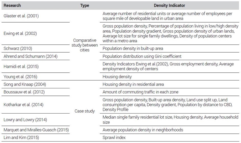
Researchers measure urban density, using various metrics such as gross population density, net population density, housing density, land use, employment density, and population density gradient (see Table 1). The most popular one is population density, either as gross density or net density (Ewing et al., 2002; Kotharkar et al., 2014; Hamidi et al., 2015). Among those, Galster et al. (2001) claimed that housing density is most effective; and it has been used in numerous studies (Song and Knaap, 2004; Lowry and Lowry, 2014; Young et al., 2016). While some studies relied on a single indicator to measure density, others developed an index consisting of various indicators (Ewing et al., 2002; Hamidi et al., 2015).

The list of density indicators
Interpreting density requires caution since the same level of density can have a quite different urban forms. In the case of large cities, the results may be distorted as sprawl is likely to be underestimated in a polycentric or dispersed city (Yang et al., 2018). Also, the sprawl index derived from population density has limitations in detecting leap frog deveolopment pattern (Lim and Kim, 2015). Nevertheless, density holds significance in explaining commuting characteristics in urban areas. High density cities show common features including lower per capita vehicle ownership, shorter total distance traveled per person and average commute time, and higher share of public transport and walking in transport mode choice (Ewing, 2002; Hamidi et al., 2015). The increase in urban density reduces transportation costs including gasoline and parking costs (Young et al., 2016). On the other hand, a few studies argue that higher density and urban compactness could slightly shorten trip lengths, but the higher travel frequency attenuates the effect (Duranton and Turner, 2018).
Looking at the urban form from various perspectives was mainly developed in previous studies on urban sprawl. In a study of urban forms in U.S. cities, Galster et al. (2001) defined sprawl based on eight dimensions of land use patterns: density, continuity, concentration, clustering, centrality, nuclearity, mixed use, and proximity. Ewing et al. (2002) associated sprawl with low-density development, complete separation of homes, shops, workplaces, lack of thriving activity centers, and limited transportation choices. They also developed a sprawl index consisting of four factors, residential density, neighborhood mix, strength of activity centers, and accessibility. Later, Ewing and Cevero (2010) expanded the index incorporating seven dimensions: density, diversity, design, demand management, accessibility to destination, distance to public transport, and demographic characteristics. Lowry and Lowry (2014) specified the four dimensions of urban form as density, centrality, accessibility, and neighborhood mix.
Given the complex relationships between various urban form factors, research focusing only on density may not be as accurate. According to Ewing (2002), high population density is related to mixed land use and accessibility as measured based on road networks, but not related to centrality. A study of 28 European countries showed no relationship between population density and compactness index (Xu et al., 2019).
Urban proximity is recognized as a highly important domain in compact city research. Distances traveled to access urban functions and services are major indicators for sustainable urban forms and mobility (Marquet and Miralles-Guasch, 2015). In adittion, urban proximity contributes to urban growth (Ahrend and Schumann, 2014; Gomes et al., 2018; Kasraian et al., 2019) in that a change in distance to activity centers, proxy for urban proximity, affects the level of total trip length, and choice of walking and public transport, greater than with a change in population density (Ewing and Cervero, 2010). Indeed, proximity plays an important role in urban compactness, and we need to explore the relationship between density and proximity, which maynot be always complementary.
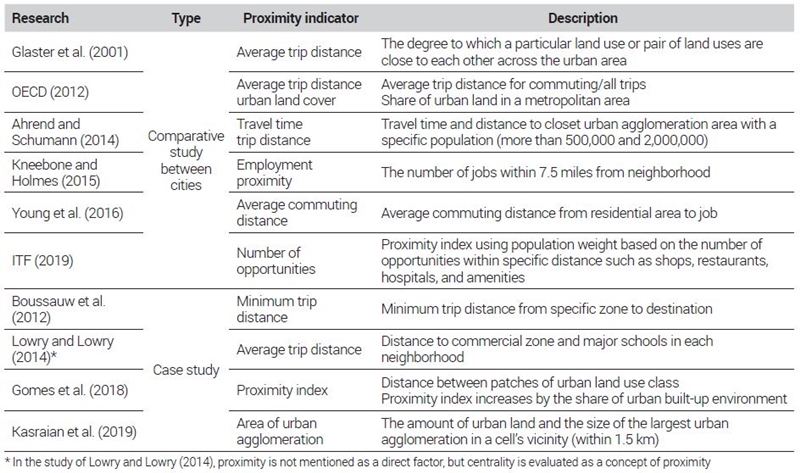
Researchers have used different definitions, approaches, and indicators in examining urban proximity. The most popular indicator for proximity is indicators related to trip distance (see Table 2). Galster et al. (2001) defined proximity as the degree to which different land uses are close to each other, and calculated the proximity of urban activities using the average distance between different land uses. The OECD (2012) defined proximity as the nearness of urban activities to other activities throughout urban areas. They suggest that trip distances traveld is the best proxy for proximity, where a shorter average trip distance indicates greater urban agglomeration.
The list of proximity indicators
Marquet and Miralles-Guasch (2015) included spatiotemporal features in the concept of proximity, while Boussauw et al. (2012) related proximity to high density, mixed land use, and small housing lots. Young et al. (2016) measured proximity based on average trip distance, and analyzed the its potential effects on transportation costs. Ahrend and Schumann (2014) measured proximity in terms of distance to areas of urban agglomeration and trip distance to analyze the relationship between spatial patterns of European economic growth and proximity.
While Lowry and Lowry (2014) did not fully specify the concept of proximity, they argues that it is closely related to centrality. Among research on urban proximity that took into account physical features, Kasraian et al. (2019) measured proximity using the size of the largest urban agglomeration in a cell’s vicinity, and defined accessibility in terms of trip distance and time to transport infrastructure. In fact, many have used urban proximity interchangeably with accessibility. Kneebone and Holmes (2015) analyzed proximity using the number of jobs within the average trip distance from residential areas. ITF (2019) also considers proximity as an indication of the degree of spatial concentration between the starting point and destination of traffic, measuring the number of services provided within a specific distance from the center of the urban grid cell (schools, hospitals, grocery stores, restaurants, leisure activities, parks, etc.).
3. Relationship between Urban Density and Proximity
Most research on urban forms has identified morphological characteristics and analyzed their effects on environment or economic growth. However, the relationship between the morphological characteristics, including urban density and proximity, was largely overlooked. The OECD (2012) study is one of the few that discusses the density-proximity relationship. It emphasizes that a compact city shall be dense and proximate, demonstrating the two are not necessarily complementary as shown in Figure 1. The figure shows that urban form in a) and c) have the same density, but the proximity in c) is twice that of a). That is, c) has a shorter average trip distance between homes and urban activities, leading to lower transport costs.

Urban density and proximity in neighborhood and city scale (OECD, 2012)Note: The circles are urban settlements consisting of residents and jobs
Other than the OECD (2012) study, Marquet and Miralles-Guasch (2015) found that higher population density increases the number of short distance trips, but the results were not significant above a certain density. Boussauw et al. (2012) analyzed spatial proximity using minimum commuting distance as an indicator of proximity, and verified the strong relationship between residential density and short commute, and between job density and long commute. Given the lack of research on the relationship between urban density and proximity, this study seeks to perform an in-depth analysis of the density-proximity relationship in global cities.
Ⅲ. Research Scope and Methodology
1. Scope of Research
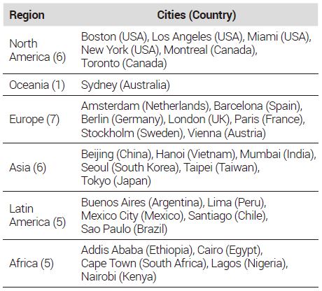
For the analysis, this study reviewed cities included in the Sustainable Cities Index, Global Cities Index, and Green City Index, and selected commonly listed cities as candidates. We have included relatively similar number of cities by continent and capital cities for the major country. The final cities for analysis were determined considering their diversity, population, economy, and development status (see Table 3 and Figure 2). The spatial range of cities for the analysis was set based on their functional boundaries, not administrative boundaries. The most recent data was retrieved, with NTL data dating to April 2019, and POI data to February 2020.
The list of 30 cities used in analysis

Distribution of cities for our analysis
2. Data
As a global comparative study, aquring common data for all cities of our interest is essential. To overcome data availabiliy issue, this study uses open source data such as OpenStreetMap (OSM) data, specifically its POI (Point of Interest), road networks and building data. OSM allows users to edit and update maps, and offers real-time map data at a global level. OSM has been used in various research on land use and land cover mapping (Zhou et al., 2019), tracking of urban changes (Zhang and Pfoser, 2019), measurement of land use diversity (Yue et al., 2017), and production of rural accessibility maps (World Bank, 2019). Many studies have also assessed OSM data’s reliability and appropriateness, concluding that they are accurate and valuable for urban science research (Touya et al., 2017; Zhang and Pfoser, 2019). In terms of POI data, a tool to measure accessibility to POI was developed by the World Bank (2019) using OSM road network data and POI. POI data is closely related to human lives, and has enormous potential (Lu et al., 2020). POI refers to key facilities, stations, schools, accommodation, restaurants, and shops that are marked on electronic maps. OSM data includes various facilities, and POI has been used as an indicator of urban activity centers.
Night Time Light (NTL) data is a measurement of city lights at night using artificial satellites. It is closely related to income and socioeconomic activities (Li and Zhou, 2017). Among NTL data, we used Visible Infrared Imaging Radiometer Suite (VIIRS) data for April 2019.
WorldPop population grid data was used to measure population density by city. WorldPop estimates population using a random forest model comprised of topographical data, Globcover Landcover, GPW v4, Landsat, OSM, and commuting time (Lloyd et al., 2017). WorldPop data is available as public data and in grid cells with a high resolution of 100 m. Annual population data is provided by country for 2000 to 2020.
United States Geological Survey (USGS) provides MODIS land cover data for the entire world. MCD12Q1 v006 (MODIS/Terra+Aqua Land Cover Type Yearly L3 Global 500 m SIN Grid) presents annual land cover data from 2001 to 2018 in 500 m grid units, and this study uses the built-up area band included under Land Cover Type 1, except African continent. We found that MODIS data for the continent has some erros, thus Copernicus data was used instead. Copernicus provides land cover data at 100 m resolution from 2015 to 2018. Cells with an urbanization ratio exceeding 30% were classified as urban areas, as was used for MODIS land cover data. This study used land cover data dating to 2018.
3. Methodology
The research flow is presented in Figure 3. The process consists of four steps: identifying urban areas using NTL, measuring proximity using POI, measuring density, and comparing the density-proximity relationship.

Research flow
Urban activities occur at a regional level where multiple cities interact. Thus, traditional administrative boundary of a city cannot accurately capture real-world relationships (Berdegué et al., 2019). Since proximity in this study is related to mobiliy, our spatial boundary should coincide with a functional area, not a city’s administrative boundary. In this context, NTL has vast potential in identifying a region(Li and Zhou, 2017), and has been widely used in relevant research to identify functional urban areas (Dou et al., 2017; Xue et al., 2018; Berdegué et al., 2019). Using NTL data, we can identify areas which are brighter than surroundings at night (Henderson et al., 2003) including conurbation boundaries (Berdegué et al., 2019).
When using NTL, setting appropriate criteria is critical for distinguishing between urban and rural regions since threshold values determine boundaries (Henderson et al., 2003; Li and Zhou, 2017). However, due to NTL data’s blooming effect, light from urban areas diffuses to non-urban areas, making it difficult to set accurate criteria. Each country and city needs different threshold values considering its environment and socioeconomic characteristics (Li and Zhou, 2017; Xue et al., 2018). This study adopts the method of Dou et al.(2017), who derived threshold values of NTL from land cover classification types using Cohen’s kappa coefficients, which measures the inter-rater reliability for categorical items. Zhou et al. (2015) used kappa coefficients to compare NTL-based urban areas to urban areas identified using MODIS, GlobGover, GLC2000, and GRUMP.
This study calculated NTL threshold values by city, using MODIS and Copernicus land cover data. Using the built-up area classification, the NTL value with the largest kappa coefficient was set as the threshold (see Eq. 1). The initial spatial scope for urban area identification was set as the main city and area within the maximum travel distance of 60km from the city center as proposed by Gerten et al. (2019).
| (1) |
This study applied the region-growing algorithm by Wicht and Kuffer (2019) and Angel et al. (2005), which merges segments with similar values into adjacent urban areas, to identify urban area boundaries. In this study, we classified empty areas within cities and continuous areas within a 1km radius as urban areas, as proposed by Wicht and Kuffer (2019) and Angel et al. (2005).
This study defined proximity as the “network distance to the urban activity center per person.” While most studies measuring urban proximity or accessibility rely solely on POI data (ITF, 2019; World Bank, 2019), its accuracy varies by region. To overcome the limitation, this study identified urban activity centers using POI density and measures proximity by calculating the actual network distance to the urban activity center by weighting the population. POI has been widely used to identify activity centers of cities (Lou et al., 2019; Deng et al., 2019; Lu et al., 2020).
In our study, urban activity centers were identified using NTL, POI, Local Moran’s I, and Geographically Weighted Regression (GWR) suggested by Lou et al. (2019). The advantage of classifying basic zones with NTL data is that it enhances the accuracy of identifying urban activity centers based on POI density (Lou et al., 2019). This study used VIIRS NTL data via the Qgis-Grass GIS Plugin, separated raster images under the region growing algorithm, and set the separated areas as basic zones. And then, population and POI density were calculated using the generated basic zones as the analysis unit.
We derived two types of urban centers, main centers and sub-centers. The main centers were identified using the Anselin Local Morans’ I statistics, one of the spatial cluster analysis techniques, using the base area’s POI density calculated previously. Local Morans’ I is a technique that identifies regions with statistical differences compared to surrounding regions by local spatial autocorrelation (Kang, 2008). This study calculated Local Moran’s I with POI density, and identified the main centers as high-high clusters, which are surrounded by regions of similarly high density. On the other hand, sub-centers were identified using the residual of GWR. They are areas with a relatively higher density than others. We conducted GWR with POI density as a dependent variable and distance from basic zone to the main center as an independent variable. A positive residual indicates a local increase in POI density (Lou et al., 2019), and basic zones having a residual value of at least 2.58 were set as sub-centers.
Urban proximity, the network distance to the nearest urban activity center from each basic zone, was calculated using Python OSMnx and NetworkX packages using population as a weight (Eq. 2). The total distance traveled by citizens was standardized to allow comparison across cities.
| (2) |
The city’s population density was calculated using World Pop population data. In this study, the density is derived as total population per urbanized area, net density (Eq. 3). An urban area is the one exceeding the threshold urban boundary of NTL with more than three people per ha, following Dijkstra et al. (2018).
| (3) |
We invested the density-proximity relationship by drawing a scatter plot using density and proximity values by city. The criteria proposed by IMF (2020) was used to determine whether a city belonged to a developing country or a developed country. Finally, the difference in the density-proximity relationship between developed and developing countries was investigated.
Ⅳ. Analysis Results
1. Identification of Urban Areas
This study identified urban areas for each city using NTL data and land cover data to establish its spatial analysis scope. The identified regions show a very different pattern from the city’s administrative boundary and capture its functional relationship. The average size of the 30 regions is 2,235.3 km2, which is 3.7 times Seoul’s administrative area. By continent, North America (3,942.5 km2), Asia (2,985.5 km2), Australia (1,784.2 km2), South America (1,745 km2), Africa (1,284.9 km2), Europe (1,222.5 km2) showed the largest scale in the order of the region area. It is noteworthy that the average size of urban areas in North America and Europe differs by more than three times. North American cities such as New York (8,475 km2), LA (5,565 km2), and Boston (3,740 km2) were far larger than major European cities such as Paris (1,919 km2) and London (2,717 km2). It can be understood that this is because the metropolitan area of the United States is more horizontally spread than the metropolitan area of Europe. When comparing the population of the corresponding urban area, New York (18.9 million), LA (14.2 million), and Boston (4.7 million), Paris (10.8 million), and London (12.1 million) appear in order, showing that large cities in the United States have a very low density compared to the size of the urban area.
In the meantime, we found that there exists a big difference between the urban area boundary derived in this study and the actual administrative boundary of the corresponding city. As shown in Figure 4, 22 cities had boundaries larger than their administrative boundaries. Except for Beijing, 29 cities had an average area of 2,181 km2, which is almost two times larger than the average administrative boundaries (1,184 km2). These results suggest that the analysis at the level of urban administrative districts may not accurately reflect the regional-level activities, which occupies a majority of urban activities. In modern cities, where the activity radius is gradually widening due to mobility improvement, it is necessary to establish functional boundaries to study urban activities.

Administrative area vs. Metropolitan area
A comparison of the regional population derived in our study and population data from Demographia 20191 confirmed the validity of the identified regions in the study. Demographia estimates the population for 1,050 urban areas with a population of 500,000 or more each year. The average population of the 30 cities was similar at 11.05 million in our study and 11.44 million in Demographia, and the standard deviation of the population was 11.7%. Therefore, we can conclude that the population size of the uban areas extracted using NTL data was also reasonable.
2. Basic Features of Cities
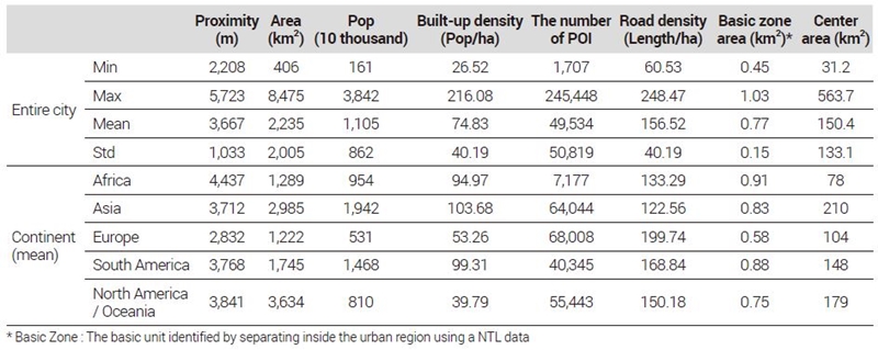
Proximity, one of the critical elements examined in this study, averaged 3,667m for the 30 cities studied (see Table 4). The cities with high proximity were Paris (2,208 m), Taipei (2,414 m), Lima (2,437 m), Vienna (2,269 m), and London (2,557 m) in the order, and those with low proximity were Lagos (5,723 m), Montreal (5,346 m), and Cairo (5,282 m). European cities such as Paris show high proximity, indicating good accessibility to urban centers. On the other hand, the low proximity in African cities such as Lagos implies poor accessibility from residential areas to urban centers. Given the poor traffic conditions, actual proximity levels in real life is expected to decrease further. Figure 5 shows the proximity distribution of Paris and Lagos to compare two extreme cases. The proximity of the entire population in Lagos is much lower than in Paris, which can be explained by the mismatch between the distribution of urban centers and the population in Lagos.
Summary statistics about status of cities (urban area)

Total distance to urban centers in Paris and Lagos on each basic zoneNote: Total Distance : Distance to urban center from each basic zone×Population in each basic zone (km×pop)
Meanwhile, the cities with high density were Mumbai (216 people/ha), Cairo (147 people/ha), Mexico City (133 people/ha), and Seoul (114 people/ha), while those with low density were Boston (27 people/ha), Miami (31 people/ha), and Amsterdam (33 people/ha). When compared by continent, the density of urban areas in Asia, Latin America and Africa are twice as high as those in Europe, North America, and Australia. The cities with the highest density in Europe and North America fall short of density levels in Asia, Latin America, and Africa. Thus, the varying levels of urban proximity and density by continent should be considered with care in understanding the compact city model.
Cities with the largest populations are Tokyo (38.4 million), Beijing (24.8 million), and Seoul (22.42 million), which are all located in Asia. On the other hand, European cities’ urban population size was the smallest, while their urban road density is the highest among contingents. While the number of POI varies significantly by city, the urban centers identified using POI are more closely associated with POI density than the absolute number of POI.
3. Density-Proximity Relationship
Figure 6 shows the scatter plot for the density-proximity relationship of the 30 cities studied. The x-axis represents urbanization density, and the y-axis represents urban proximity. In addition to the density-proximity regression line, a thin dotted line shows the average density and proximity of cities. The size of the nodes is proportionate to population size. The figure shows that overall urban proximity tends to deteriorate as the density increases, which contradicts the compact city’s previous discussions that argued that density and proximity are complementary.

Urban proximity vs. density
Cities can be divided into four groups based on their density and proximity compared to the global average to understand their characteristics better.
The high-density and poor-proximity cities in the first quadrant include Mumbai, Cairo, Mexico City, and Sao Paulo, all from developing countries. In these cities, the population center is likely to be different from the urban center. Low-density and poor-proximity cities in the second quadrant are the weakest in terms of compact city traits and have a high possibility of exhibiting urban sprawl, making them the least sustainable urban among the four groups. The third quadrant cities have low density but good proximity, meaning that urban activities can be easily accessible despite the low density. This group includes European cities such as Paris, London, Vienna, and some Asian cities such as Tokyo and Taiwan. Lastly, the cities in the fourth quadrant have high density and good proximity, which is the most ideal given the definition of the compact ciy concept. Even among the high-density and good-proximity cities, Seoul shows a remarkable difference, with a population density 40 people/ha higher than the average. The results show that Seoul is highly competent in urban compactness even when compared to global cities.
However, the above classification is based on the relative density and proximity of the cities included in this study; and is not an explicit criterion for judging the compactness of a city. We have to acknowledge that the average density and proximity levels derived in Figure 6 may surpass or fall short of ideal values. Since it is difficult to determine the ideal density and ideal proximity, this study used average values as a criterion.
Figure 6 shows that the relationship between density and proximity is negative, but we might need to investigate the relationship considering their respective characteristics. For instance, Western cities’ density except for Barcelona in Western countries is below average (75/ha), and cities exhibit different density tendencies by continent. Thus, this study classifies cities into developed and developing countries and analyzes the density-proximity relationship between the two groups (Figure 7 and Figure 8). The analysis revealed apparent differences in density-proximity relationship and urban compactness between the two groups.

Scatter plot of urban proximity and density in developed country’s cities

Scatter plot of urban proximity and density in developing country’s cities
In developed countries (17 cities), urban proximity improved with increasing density, which coincides with the existing literature. Urban centers in developed countries are compact and dense, and the analysis of population distribution and distance to urban centers showed that most citizens reside near the centers. The average density and proximity of cities in developed countries were 53 people/ha and 3219m. European cities generally had higher proximity, including Paris, Vienna, and London. North American cities except Toronto have lower density and proximity. The results demonstrate the urban sprawl phenomenon of American cities and the compactness of European cities. Compared to other cities in developed countries, Seoul has a much higher urban density, more than twice the average density, and is also highly ranked in proximity. Its density is double that of the neighboring Asian city of Tokyo, although the two cities had similar proximity levels.
On the other hand, Figure 8 shows that thirteen cities in developing countries exhibit patterns different from developed countries. Urban density and proximity are negatively related, which implies that the dense urban environment is not always a compact urban form. Compared to developed countries, the average proximity is poor by 1,000 m, indicating significant differences between urban centers and residential centers. The average density and proximity are 104 people/ha and 4,253 m. That is, density is two times higher, while proximity is poorer than in developed countries.
The differences in the density-proximity relationship between developing countries and developed countries can be thought of in connection with urban spatial features. We calculated a Gini coefficient, an indicator widely used to measure urban spatial structures, to analyze the level of inequality in POI density distribution. The average Gini coefficient of developed countries is 0.69, while that of developing countries is 0.77, demonstrating that the inequality in the distribution of urban activities is more severe in developing countries. The Gini coefficient is the highest in the order of Lagos (0.92), Beijing (0.89), Cairo (0.88), Hanoi (0.87), and Nairobi (0.85). For the case of developing countries, POIs are concentrated in a few specific areas, having negative effects on proximity. As such, cities in developing countries show more significant mismatch between where people reside and activity centers. The population living within 1 km of urban centers is 23% for developed countries and 19% for developing countries, and those living further than 5 km amount to 20% and 30% of the total population, respectively. Thus, a significant proportion of the population in developing countries is living far away from urban centers. In the case of developed countries, population centers are relatively close to activity centers, and urban activities are relatively decentralized.
Figure 9 contrasts the difference between developed countries and developing countries. As shown, cities with high density have a higher proportion of the population distributed near activity centers in developed countries. It is likely that the higher the density, the stronger the attraction to the city center where urban functions are concentrated for economic and social activities with urban amenities. On the other hand, developing countries show a clear difference between the distribution of POI density and the distribution of population density. Besides, a large proportion of the population resides in the city’s outskirts, away from urban centers. The level of economic growth and urban development seems to influence the density-proximity relationship, which might be related to slums in developing countries.

POI and population distribution in developed and developing countryNote: Density of city on right is higher than left one in each class
To conclude, for cities of developed countries, urban activity centers are relatively uniformly distributed and populations are densely located in the activity centers, so an increased density can improve proximity. On the other hand, an increase in population density can worsen proximity in developing countries because activity centers are concentrated at specific points and people tend to live further away from activity centers.
Ⅴ. Conclusions and Policy Implications
This study examined the density-proximity relationship, a key characteristic of the compact city, and analyzed differences in compact city features between developed and developing countries. We proposed a framework utilizing NTL data and OSM POI data to extract compact city characteristics of global cities. The major findings of this study are as follows.
First, the identified urban areas using NTL and land cover data are about two times larger than administrative city boundaries. The result indicates that functional urban areas are more appropriate analysis units in analyzing urban activities, considering the improved mobility and active interactions between the central and surrounding cities.
Second, urban density and proximity are intertwined, but in different directions depending on whether cities belonged to developing or developed countries. In the case of developed countries, higher density led to improved proximity. This observation is consistent with the existing literature. However, we found that increases in density in developing countries somewhat deteriorate proximity. A comparison of the Gini coefficient and population density showed that urban centers in developing countries are more concentrated at a few specific areas, while populations are concentrated away from the centers. Therefore, the results imply that different methods must be sought according to cities’ economic, technological, socio-cultural characteristics to improve proximity.
Third, the density and proximity characteristics of cities are clearly different by region. In particular, North American cities are characterized by low-density development, while European cities have high proximity but various density levels. Dense development may be preferred for efficiency reasons, but the ideal compact city model may be considered one with low/medium density and high proximity as high density derives more vulnerabilities, especially in the post-coronavirus pandemic.
The limitation of this study is that the analysis result is inevitably affected by the amount, accuracy and reliability of the POI data. Due to the nature of the OSM platform, data cannot be the same in all cities. Nevertheless, this study's significance lies in proposing a framework applicable to all cities and utilizing various sources as expected of the era of big data to examine the density-proximity relationship and recommend directions for the compact city model. The non-linear patterns in the relationship between density and proximity depending on city characteristics highlight the need for follow-up research on the density-proximity relationship’s influencing factors.
Acknowledgments
This study was supported by the SNU New Faculty Research Settlement Fund and National Research Foundation of Korea (No. NRF-2017R1C1B1004785) funded by the Ministry of Science & ICT.
References
- Ahrend, R. and Schumann, A., 2014. Does Regional Economic Growth Depend on Proximity to Urban Centres?, Paris: OECD.
- Angel, S., Sheppard, S., Civco, D.L., Buckley, R., Chabaeva, A., Gitlin, L., Kraley. A., Parent. J., and Perlin, M., 2005. The Dynamics of Global Urban Expansion, Washington: World Bank.
-
Berdegué, J.A., Hiller, T., Ramírez, J.M., Satizábal, S., Soloaga, I., Soto, J., Uribe, M., and Vargas, O., 2019. “Delineating Functional Territories from Outer Space”, Latin American Economic Review, 28(1): Article No. 4.
[https://doi.org/10.1186/s40503-019-0066-4]

-
Bhatta, B., Saraswati, S., and Bandyopadhyay, D., 2010. “Urban Sprawl Measurement from Remote Sensing Data”, Applied Geography, 30(4): 731-740.
[https://doi.org/10.1016/j.apgeog.2010.02.002]
-
Boussauw, K., Neutens, T., and Witlox, F., 2012. “Relationship between Spatial Proximity and Travel-to-work Distance: the Effect of the Compact City”, Regional Studies, 46(6): 687-706.
[https://doi.org/10.1080/00343404.2010.522986]
-
Boyko, C.T. and Cooper, R., 2011. “Clarifying and Re-conceptualising Density”, Progress in Planning, 76(1): 1-61.
[https://doi.org/10.1016/j.progress.2011.07.001]
-
Burton, E., 2002. “Measuring Urban Compactness in Uk Towns and Cities”, Environment and Planning B: Planning and Design, 29(2): 219-250.
[https://doi.org/10.1068/b2713]
-
Burton, E., Jenks, M., and Williams, K., 2003. The Compact City: A Sustainable Urban Form?, London: Routledge.
[https://doi.org/10.4324/9780203362372]
-
Creutzig, F., Lohrey, S., Bai, X., Baklanov, A., Dawson, R., Dhakal, S., Flamb, W., McPhearson, T., Minx, J., Munoz, E., and Walsh, B., 2019. “Upscaling Urban Data Science for Global Climate Solutions”, Global Sustainability, 2: 1-25
[https://doi.org/10.1017/sus.2018.16]
- Dantzig, G.B. and Saaty, T.L., 1973. Compact City: a Plan for a Liveable Urban Environment, New York: WH Freeman.
-
Deng, Y., Liu, J., Liu, Y., and Luo, A., 2019. “Detecting Urban Polycentric Structure from POI Data”, ISPRS International Journal of Geo-Information, 8(6): 283.
[https://doi.org/10.3390/ijgi8060283]
-
Dieleman, F. and Wegener, M., 2004. “Compact City and Urban Sprawl”, Built Environment, 30(4): 308-323.
[https://doi.org/10.2148/benv.30.4.308.57151]
- Dijkstra, L., Florczyk, A., Freire, S., Kemper, T., Pesaresi, M., and Schiavina, M., 2018. “Applying the Degree of Urbanisation to the Globe: A New Harmonised Definition Reveals a Different Picture of Global Urbanisation”, Paper presented in Proceedings of the 16th IAOS Conference: Better Statistics for Better Lives, Paris: OECD Headquarters.
-
Dou, Y., Liu, Z., He, C., and Yue, H., 2017. “Urban Land Extraction Using VIIRS Nighttime Light Data: An Evaluation of Three Popular Methods”, Remote Sensing, 9(2): 175.
[https://doi.org/10.3390/rs9020175]
-
Duranton, G. and Turner, M.A., 2018. “Urban Form and Driving: Evidence from US Cities”, Journal of Urban Economics, 108: 170-191.
[https://doi.org/10.1016/j.jue.2018.10.003]
- Ewing, R.H., Pendall, R., and Chen, D.D., 2002. Measuring Sprawl and Its Impact, Washington, DC: Smart Growth America.
-
Ewing, R. and Cervero, R., 2010. “Travel and the Built Environment: A Meta-analysis”, Journal of the American Planning Association, 76(3): 265-294.
[https://doi.org/10.1080/01944361003766766]
-
Galster, G., Hanson, R., Ratcliffe, M.R., Wolman, H., Coleman, S., and Freihage, J., 2001. “Wrestling Sprawl to the Ground: Defining and Measuring An Elusive Concept”, Housing Policy Debate, 12(4): 681-717.
[https://doi.org/10.1080/10511482.2001.9521426]
-
Gerten, C., Fina, S., and Rusche, K., 2019. “The Sprawling Planet: Simplifying the Measurement of Global Urbanization Trends”, Frontiers in Environmental Science, 7: 1.
[https://doi.org/10.3389/fenvs.2019.00140]
-
Gomes, E., Banos, A., Abrantes, P., and Rocha, J., 2018. “Assessing the Effect of Spatial Proximity on Urban Growth”, Sustainability, 10(5): 1308.
[https://doi.org/10.3390/su10051308]
-
Hamidi, S., Ewing, R., Preuss, I., and Dodds, A., 2015. “Measuring Sprawl and Its Impacts: An Update”, Journal of Planning Education and Research, 35(1): 35-50.
[https://doi.org/10.1177/0739456X14565247]
-
Henderson, M., Yeh, E.T., Gong, P., Elvidge, C., and Baugh, K., 2003. “Validation of Urban Boundaries Derived from Global Night-time Satellite Imagery”, International Journal of Remote Sensing, 24(3): 595-609.
[https://doi.org/10.1080/01431160304982]
- IMF (International Monetary Fund), 2020. World Economic Outlook, April 2020: The Great Lockdown.
- ITF (Internation Transport Forum), 2019. “Benchmarking Accessibility in Cities: Measuring the Impact of Proximity and Transport Performance”, International Transport Forum Policy Papers, 68: 1-83.
- Jenks, M.J., Burgess, M.J.R., Acioly, C., Allen, A., Barter, P.A., and Brand, P., 2000. Compact Cities: Sustainable Urban Forms for Developing Countries. Abingdon-on-Thames: Taylor & Francis.
-
Jeong, Y.H. and Lee, J.H., 2013. Study on Current Status and Prospects of Compact City Policies in Korea, Anyang: Korea Research Institute for Human Settlements.
정윤희·이진희, 2013. 「한국 컴팩시티 정책의 현황 및 과제 연구」, 안양: 국토연구원. -
Jo, Y.A. and Choi, M.H., 2013. “Empirical Study on the Optimum Urban Density for 74 Autonomous Districts of the Metropolitan Cities”, The Korean Journal of Local Government Studies, 17(3): 47-66.
조윤애·최무현, 2013. “압축도시와 적정 개발밀도에 관한 실증연구: 74개 광역시 자치구를 중심으로”, 「지방정부연구」, 17(3): 47-66. -
Kang, H.J., 2008. “Hot Spot Analysis: Basis of Spatial Analysis, Utilization and Understanding of Local Moran’s I and Nearest Neighbor Analysis”, Planning and Policy, (324): 116-121.
강호제, 2008. “핫스팟 분석기법(Hot Spot Analysis): 공간분석의 기초, 최근린군집분석과 국지모란지수의 이해와 활용”, 「국토」, (324): 116-121. -
Kasraian, D., Maat, K., and van Wee, B., 2019. “The Impact of Urban Proximity, Transport Accessibility and Policy on Urban Growth: A Longitudinal Analysis over Five Decades”, Environment and Planning B: Urban analytics and City Science, 46(6): 1000-1017.
[https://doi.org/10.1177/2399808317740355]
-
Kim, B.S. and Moon, T.H., 2011. “A Study on the Effects of Land Use Characteristics of Compact City on CO2 Emission”, Journal of Environmental Policy and Administration, 19(2): 101-115.
김병석·문태훈, 2011. “압축도시의 토지이용 특성이 이산화탄소 배출에 미치는 영향”, 「환경정책」, 19(2): 101-115. - Kneebone, E. and Holmes, N., 2015. “The Growing Distance between People and Jobs in Metropolitan America”, Metropolitan Policy Program The Brookings, 2015: 1-25.
-
Ko, E.J. and Lee, K.H., 2013. “Effects of Compact City Development on Residents’ Shopping Trips – A Case study of Seoul”, Journal of the Korea Academia-Industrial cooperation Society, 14(8): 4077-4085.
[
https://doi.org/10.5762/KAIS.2013.14.8.4077
]
고은정·이경환, 2013. “압축도시 계획요소가 지역주민들의 쇼핑통행에 미치는 영향 –서울시를 대상으로”, 「한국산학기술학회 논문지」, 14(8): 4077-4085. -
Kotharkar, R., Bahadure, P., and Sarda, N., 2014. “Measuring Compact Urban Form: A Case of Nagpur City, India”, Sustainability, 6(7): 4246-4272.
[https://doi.org/10.3390/su6074246]
-
Lee, W.K., 2014. “Compact Development for Urban Revitalization”, BDI Focus, (246): 1-12.
이원규, 2014. “도심 활성화를 위한 컴팩트시티 개발”, 「BDI 포커스」, (246): 1-12. -
Li, X. and Zhou, Y. 2017., “Urban Mapping Using DMSP/OLS Stable Night-time Light: a Review”, International Journal of Remote Sensing, 38(21): 6030-6046.
[https://doi.org/10.1080/01431161.2016.1274451]
-
Lim, S.J. and Kim, K.Y., 2015. “Evaluating Characteristics of Sprawl Index based on Population Density as a Measure of Urban Sprawl”, Journal of the Korean Urban Geographical Society, 18(2): 67-79.
임수진·김감영, 2015. “도시 스프롤 측정 방법으로서 밀도 기반 스프롤 지수 특성 평가”, 「한국도시지리학회지」, 18(2): 67-79. -
Lloyd, C.T., Sorichetta, A., and Tatem, A.J., 2017. “High Resolution Global Gridded Data for Use in Population Studies”, Scientific Data, 4(1): 1-17.
[https://doi.org/10.1038/sdata.2017.1]
-
Lou, G., Chen, Q., He, K., Zhou, Y., and Shi, Z. 2019. “Using Nighttime Light Data and Poi Big Data to Detect the Urban Centers of Hangzhou”, Remote Sensing, 11(15): 1821.
[https://doi.org/10.3390/rs11151821]
-
Lowry, J.H. and Lowry, M.B., 2014., “Comparing Spatial Metrics That Quantify Urban Form”, Computers, Environment and Urban Systems, 44: 59-67.
[https://doi.org/10.1016/j.compenvurbsys.2013.11.005]
-
Lu, C., Pang, M., Zhang, Y., Li, H., Lu, C., Tang, X., and Cheng, W., 2020. “Mapping Urban Spatial Structure Based on Poi (point of Interest) Data: A Case Study of the Central City of Lanzhou, China”, ISPRS International Journal of Geo-Information, 9(2): 92.
[https://doi.org/10.3390/ijgi9020092]
-
Marquet, O. and Miralles-Guasch, C., 2015. “The Walkable City and the Importance of the Proximity Environments for Barcelona’s Everyday Mobility”, Cities, 42: 258-266.
[https://doi.org/10.1016/j.cities.2014.10.012]
-
Neuman, M. 2005. “The Compact City Fallacy”, Journal of Planning Education and Research, 25(1): 11-26.
[https://doi.org/10.1177/0739456X04270466]
- OECD, 2012. “Compact City Policies: A Comparative Assessment”, OECD Green Growth Studies, 1-287.
-
Oh, M.J. and Jeong, J.Y., 2011. “A Study on the Urban Development Direction of Overseas and Domestic Sustainable Compact City”, Journal of the Architectural Institute of Korea : Planning & Design, 27(12): 297-306.
오민준·정재용, 2011. “국내외 지속가능한 컴팩트시티형 도시개발방향에 대한 연구”, 「대한건축학회 논문집 계획계」, 27(12): 297-306. -
Schwarz, N., 2010. “Urban Form Revisited—selecting Indicators for Characterising European Cities”, Landscape and Urban Planning, 96(1): 29-47.
[https://doi.org/10.1016/j.landurbplan.2010.01.007]
-
Song, M.K., 2015. “Issues of Global Urbanization and Growth Predicting of Emerging Cities”, World & Cities, 7: 46-55.
송미경, 2015. “세계 도시화의 핵심 이슈와 신흥도시들의 성장 전망”, 「세계와도시」, 7: 46-55. -
Song, Y. and Knaap, G.J., 2004. “Measuring Urban Form: Is Portland Winning the War on Sprawl?”, Journal of the American Planning Association, 70(2): 210-225.
[https://doi.org/10.1080/01944360408976371]
-
Touya, G., Antoniou, V., Olteanu-Raimond, A.M., and Van Damme, M.D., 2017. “Assessing Crowdsourced Poi Quality: Combining Methods Based on Reference Data, History, and Spatial Relations”, ISPRS International Journal of Geo-Information, 6(3): 80.
[https://doi.org/10.3390/ijgi6030080]
- UN Habitat, 2016. World Cities Report: Urbanization and Development: Emerging Futures, Nairobi: UN Habitat.
-
Wicht, M. and Kuffer, M. 2019., “The Continuous Built-up Area Extracted from ISS Night-time Lights to Compare the Amount of Urban Green Areas Across European Cities”, European Journal of Remote Sensing, 52(Suppl 2): 58-73.
[https://doi.org/10.1080/22797254.2019.1617642]
- World Bank. 2019. Rural Accessibility Map Completion Report, Washington: World Bank.
-
Xu, C., Haase, D., Su, M., and Yang, Z., 2019. “The Impact of Urban Compactness on Energy-related Greenhouse Gas Emissions Across EU Member States: Population Density Vs Physical Compactness”, Applied Energy, 254: 113671.
[https://doi.org/10.1016/j.apenergy.2019.113671]
-
Xue, X., Yu, Z., Zhu, S., Zheng, Q., Weston, M., Wang, K., Gan, M., and Xu, H., 2018. “Delineating Urban Boundaries Using Landsat 8 Multispectral Data and VIIRS Nighttime Light Data”, Remote Sensing, 10(5): 799.
[https://doi.org/10.3390/rs10050799]
-
Yang, J.S., 2017. “Measuring Urban Sprawl by K-nearest Facility Accessibility: A Case Study of Chuncheon City”, Journal of the Korean Geographical Society, 52(4): 479-493.
양재석, 2017. “K-근접 시설 접근성을 이용한 도시 스프롤 측정: 춘천시를 사례로”, 「대한지리학회지」, 52(4): 479-493. -
Yang, J.S., Song, H.J., Kang, K.B., Gwon, M.J., and Shin, H.S., 2018. “Metropolitan Sprawl Measures Using Multi-Facility Accessibility: A Case Study of Gwangju Metropolitan Area” Journal of the Korean Urban Geographical Society, 21(1): 77-91.
[
https://doi.org/10.21189/JKUGS.21.1.6
]
양재석·송하진·강경빈·권민지·신휴석, 2018. “복합시설 접근성을 이용한 대도시권 스프롤 측정: 광주광역시권을 사례로”, 「한국도시지리학회지」, 21(1): 77-91. -
Young, M., Tanguay, G.A., and Lachapelle, U., 2016. “Transportation Costs and Urban Sprawl in Canadian Metropolitan Areas”, Research in Transportation Economics, 60: 25-34.
[https://doi.org/10.1016/j.retrec.2016.05.011]
-
Yue, Y., Zhuang, Y., Yeh, A.G., Xie, J.Y., Ma, C.L., and Li, Q.Q., 2017. “Measurements of Poi-based Mixed Use and Their Relationships with Neighbourhood Vibrancy”, International Journal of Geographical Information Science, 31(4): 658-675.
[https://doi.org/10.1080/13658816.2016.1220561]
-
Zhang, L. and Pfoser, D., 2019. “Using Openstreetmap Point-of-interest Data to Model Urban Change−a Feasibility Study”, PLoS One, 14(2): 1-34.
[https://doi.org/10.1371/journal.pone.0212606]
-
Zhou, Q., Jia, X., and Lin, H. 2019., “An Approach for Establishing Correspondence between Openstreetmap and Reference Datasets for Land Use and Land Cover Mapping”, Transactions in GIS, 23(6): 1420-1443.
[https://doi.org/10.1111/tgis.12581]
-
Zhou, Y., Smith, S.J., Zhao, K., Imhoff, M., Thomson, A., Bond-Lamberty, B., Asrar. G. M., Zhang. X., He. C., and Elvidge, C.D., 2015. “A Global Map of Urban Extent from Nightlights”, Environmental Research Letters, 10(5): 054011.
[https://doi.org/10.1088/1748-9326/10/5/054011]