A Development of Trip Generation Model by Functions of Small City Based on Mobile Origin-destination Data

1. Research Background and Purpose

Traffic demand estimation is a process that simplifies descriptive models to recognize changes in current travel behaviors and socioeconomic conditions, and predicts future traffic demands. This process is divided into four stages: trip generation, trip distribution, mode split, and network assignment (Aboelenen et al., 2021). Among these, the first stage, trip generation estimation, provides data necessary for estimating the remaining stages (trip distribution, mode split, network assignment) (Etu and Oyedepo, 2018; Mukherjee and Kadali, 2022).

Accurately estimating the trip generation is crucial because the estimated final traffic demand values in the subsequent stages can significantly vary based on the estimated trip generation. However, the traditional traffic demand models have been typically developed using survey-based data such as household travel survey data. This data suffers from low response rates and reporting errors, and due to the high cost of conducting surveys, small collected sample size can result in biased estimates, thereby showing low reliability (Bwambale et al., 2021).

Recently, with the emergence of big data collected on a persecond basis, it has become possible to identify individuals’ trip trajectories, and numerous studies have been conducted using high spatial and temporal resolution personal travel data to explore human mobility. The primary data sources used in studies on human mobility, such as navigation and mobile phone data, cover all navigation users and mobile phone subscribers, thereby enabling a comprehensive description of travel behaviors and resulting in highly reliable analysis outcomes.

Lately, there has been an emerging trend in research aimed at developing trip generation models using a type of mobile phone data known as Call Detailed Record (CDR) data. CDR data is recorded daily as long as a mobile phone is used, offering the advantage of higher temporal resolution compared to household travel survey data collected over a single day. However, the data lacks information on variables such as household details, and the data are only recorded when the mobile phone is used, resulting in spatial and temporal discontinuities within the data. This makes it difficult to capture movements when the mobile phone is not in use, which is a notable drawback (Bwambale et al., 2021).

This study utilized sightings data, which is recorded at regular intervals regardless of mobile phone usage. Such data is processed into OD (Origin-Destination) form between cell tower-based TAZs (Traffic Analysis Zones), which has higher spatial resolution compared to the conventional TAZs at town, township or neighborhood levels. Using this data, we developed a trip generation model according to the functional characteristics of small cities.

At present, the most widely used KTDB data for estimating future traffic demand applies the same trip generation model uniformly across the whole country or by major metropolitan areas. However, cities are composed of different elements, and especially in small cities, trips can be generated by specific functional elements such as tourism, industry, agriculture, and transport-inducing facilities. Consequently, to enhance the reliability of future traffic demand estimates, there is a need to develop city function-specific trip generation models, particularly focusing on small cities. In this study, to develop city function-specific trip generation models, various variables not considered in current trip generation models were explored through a literature review on trip generation model development. In addition, actual travel data and various variables from cities with specific functions like tourism, industrial, agricultural, and fishing towns were considered.

1. Past research on trip generation model development

Chang et al. (2014) utilized household travel survey data from the Seoul metropolitan area to compare the performance of various trip generation models. The model fit of different analytical models including linear regression, Tobit, Poisson, ordered logit, and category-type was compared. Variables such as household composition, household income, transportation infrastructure, demographic characteristics, regional economy, and land use were utilized in the development of the trip generation model. The analysis showed that the category-type based trip generation model exhibited the best performance, while the linear regression-based trip generation model showed an acceptable level of performance.

Usanga et al. (2020) developed a trip generation model for residential areas. The four variables were household size, household income, car ownership, and the number of employed persons per household. The results indicated that household size was the strongest factor influencing trip generation in residential areas.

Etu and Oyedepo (2018) applied both a Radial Basis Function Neural Network (RBFNN) and a multiple linear regression model to household travel survey data from the Akure region in Nigeria, comparing the fit of the two models. Independent variables used included the number of household members, number of employed household members, number of students in the household, number of household members older than age 15, and number of driver’s license holders in the household. The analysis revealed that the deep learning technique, RBFNN, had a better fit compared to the multiple linear regression model.

Sulistyono et al. (2012) estimated a household-based trip generation model for residential areas in Jember. The independent variables included the number of family members, family members working, family members attending school, income, and vehicle ownership.

Roorda et al. (2010) developed a trip generation model for specific demographic groups such as low-income households, the elderly, and single-parent families. The independent variables used were age, income level, number of household members, vehicle ownership, number of employed persons, and population density. An ordered probit model was applied to derive the model. The analysis showed that elderly travel was significantly influenced by vehicle ownership, while travel in single-parent families was affected by both vehicle ownership and employmentre-lated indicators. Conversely, travel among low-income households was less influenced by vehicle ownership and more significantly impacted by transportation infrastructure.

Aboelenen et al. (2021) identified factors affecting trip generation in residential buildings. The independent variables included household size, income level per housing unit, vehicle ownership, nationality (Qataris, non-Qataris), number of persons with a driving license, and number of employed persons and students per housing unit. A multiple linear regression model was applied as the analytical technique.

Lafta and Ismael (2022) developed a trip generation model for the Baghdad region using various statistical approaches. The independent variables consisted of gender, number of workers, population by age group, income, type of dwelling unit, ownership of dwelling unit, area of dwelling unit, and car ownership. Artificial Neural Networks (ANN) and multiple linear regression models were used as analysis techniques. The analysis indicated that trips in the Baghdad region were associated with factors such as family size, gender, number of students in the household, number of workers in the household, and car ownership, with the ANN model performing better than the multiple linear regression model.

Masoumi (2022) developed city-specific trip generation models for cities in the Middle East and North Africa region. The independent variables included gender, age, individual driving license ownership, activity as a worker or student, car ownership, number of driving licenses in the household, household income, commute mode choice, commuting distance, node-link ratio, link length, and number of accessed facilities. The results of the analysis of variance showed that the factors influencing trip generation varied from city to city. The author of the study recommended the active use of land use variables for sustainable demand estimation.

Yang et al. (2020) developed a trip generation model for the Nanjing region in China using location-based social network data and mobile phone data. The independent variables included the number of POIs, number of public transportation stations, and number of highway entrances. The analysis showed that land use-related variables had a significant impact on trip generation.

2. Research on Trip generation model development using mobile phone data

bwambale et al. (2019) developed a methodology to enhance the accuracy of trip generation estimation using CDR data, socioeconomic indicators, and GSM (Global System for Mobile Communications) data. The traffic volumes derived from the CDR data and socioeconomic information were utilized to estimate future trip generation amounts, while the travel proportions derived from GSM data were used to construct trip generation models for different socioeconomic groups.

Bwambale et al. (2021) developed a methodology to improve the accuracy of trip generation estimation by integrating OD profiles that can be extracted from CDR data with census data and household travel survey data. The model from the study showed an overall improvement in the accuracy of trip generation estimation. However, the study was limited in that the variables used in the analysis were confined to basic socioeconomic indicators such as gender and age.

Colak et al. (2015) presented a methodology that uses CDR data and population density data alone to determine the purpose of trips made by mobile phone users. They classified trip generation areas based on the frequency and timing of mobile phone trips into categories such as work and leisure, and assigned purposes to trips based on the characteristics of the selected trip generation areas.

Shi and Zhu (2019) identified the residential and employment areas of users based on mobile phone data traffic and spatial distribution. They developed Traffic Analysis Zones (TAZs) based on cell tower locations and developed models for trip generation and inflow in individual TAZs through a multiple regression analysis.

3. Research distinctiveness

First, a trip generation model for small cities based on their functions was developed. Household travel survey data typically collects travel and socioeconomic information at the eup-myeon-dong level, which is suitable for deriving trip generation models for large cities, but inadequate for rural and fishing areas in small cities due to a lack of TAZ samples. In this study, trip generation models specific to small cities were derived using cell tower-based TAZs, which have higher spatial resolution compared to the eup-myeon-dong level TAZs.

Second, a PA-based trip generation model was developed through type estimation of origins and destinations in mobile origin-destination data. Since traditional mobile phone data does not include information on the purpose of travel, only OD-based trip generation models could be derived. However, a PA-based model better represents travel patterns from a behavioral perspective compared to an OD-based model and has less aggregation error, making it preferable for estimation (Kim, 1997). This study estimated the types of origins and destinations based on mobile phone users’ travel behaviors to derive a PA-based trip generation model.

Third, a trip generation model was derived considering various variables including transportation infrastructure and land use. Traditional trip generation models used in policy-making are based on household travel survey data, which tends to focus predominantly on socioeconomic indicators. In this research, variables not considered in existing trip generation models but used in related studies, such as public transportation stops, node links, and land use variables, were utilized as independent variables.

1. Research Flow and Spatial Scope

The flow of this study is as follows. First, the spatial scope of the study was determined based on population size. Second, the concept and preprocessing of the mobile origin-destination data used in this research were explained. Third, independent variables were selected considering those used in the current KTDB and various previous studies for developing trip generation models. Fourth, analytical methods were chosen based on the characteristics of trip production and attraction in the TAZ-specific mobile origin-destination data. Fifth, key variables for the development of the trip generation model were identified through a correlation analysis, and a regression analysis was applied to develop the trip generation model.

For the development of city function-specific trip generation models, four cities were selected as spatial scopes, each differing in city functions, as shown in <Figure 1>. It was assumed that large and medium-sized cities, having complex city functions, would present limitations in constructing function-specific models. Therefore, this study focused on developing city function-specific trip generation models centered on small cities. The demographic definition of small cities was based on Yim (2019), defining them as cities with a population of less than 200,000.

Figure 1.

Study sites (polygon unit)

First, the city selected as a tourism city is Andong in Gyeongsangbuk-do. As of 2022, the population of Andong was approximately 150,000, and it has recently been selected as one of the five major tourism hubs by the Ministry of Culture, Sports and Tourism. Second, the city selected as an industrial city is Eumseong-gun in Chungcheongbuk-do. As of 2022, the population of Eumseong-gun was about 100,000, and it currently leads the industry in the central region with over 330 companies located in 16 industrial complexes. Third, the city selected as a rural city is Euiseong-gun in Gyeongsangbuk-do. As of 2022, the population of Euiseong-gun was about 50,000, and more than 30% of the total population is engaged in agriculture. Fourth, the city selected as a fishing city is Sinan-gun in Jeollanam-do. As of 2022, the population of Sinan-gun was approximately 40,000, and it is known as a representative fishing city in Korea, based on its various fishing infrastructures.

2. Mobile origin-destination data

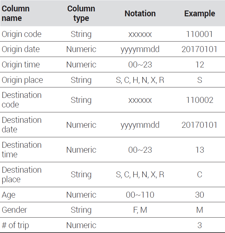
In this study, the mobile origin-destination data used for developing the trip generation model consists of data processed from the mobile phone trajectory data of KT subscribers into the form of origin-destination traffic volumes. It includes information such as origin and destination TAZ codes, time of departure and arrival, types of locations (residential or activity areas) of the origin and destination TAZs, gender, age, and traffic volumes.

The processing of mobile origin-destination data was carried out as follows (Kim et al., 2021). First, error data such as NULL values were removed and corrected from the mobile phone trajectory data. Second, movements and stays were distinguished based on a duration of stay. Third, to differentiate between origins and destinations, individual trips were sorted and spatially organized based on the date of data recording, start time of stay, and end time of stay. Finally, areas considered residential or potential activity locations were used as origins and destinations, and traffic volumes between TAZs were aggregated. The final aggregated mobile origin-destination data has the structure shown in <Table 1> (Kim and Song, 2022).

Table 1.

The dataset of mobile phone OD data (Kim and Song, 2022)

The methodology for estimating types of stay locations to extract PA-based trip production and attraction from mobile origin-destination data is as follows. Initially, if an individual traveler’s monthly trajectory data shows characteristics of staying for more than three hours between 21:00 and 07:00 on at least three days a week and three weeks a month, then that TAZ is defined as a home (H) or non-home stay area (N). Next, if an individual traveler’s monthly trajectory data shows characteristics of staying for more than three hours between 09:00 and 18:00 at least two days a week and two weeks a month, then that TAZ is defined as a workplace (C) or school (S). If the traveler is aged over 20, the location is defined as a workplace; if under 25, as a school. For those aged between 20 and 25, if these criteria are met during the vacation months of January-February and July-August, it is defined as a workplace; if not met, it is defined as a school. All other stay locations are defined as potential activity areas. Within these, TAZs where the frequency of stay occurs three or more times a week are defined as other (X) areas, and TAZs without any characteristic stay patterns are defined as religious activity areas (R).

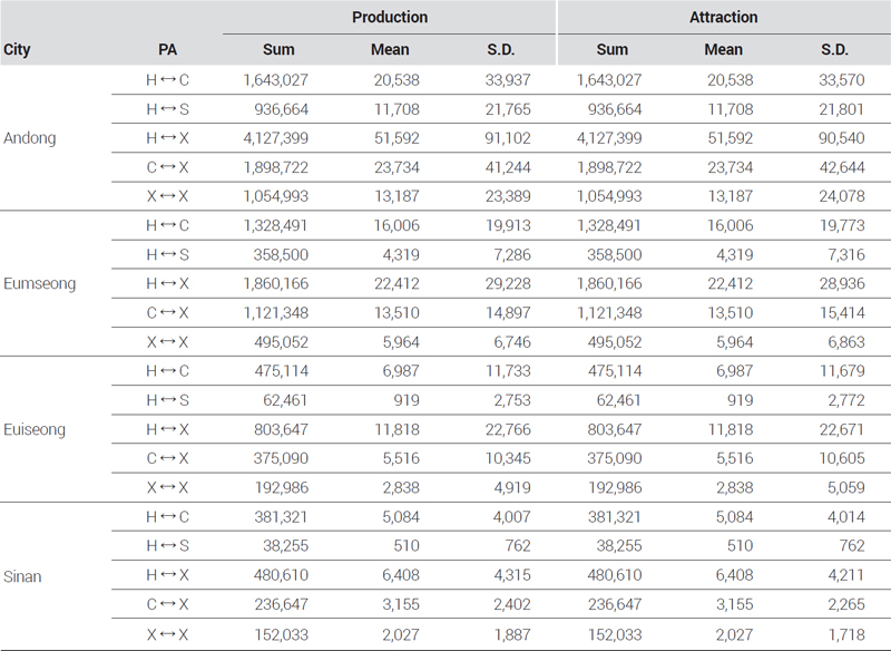
Five types of PA travel were derived based on the types of origins and destinations. First, if either the origin or destination is a home (H) or a company (C), it is defined as household-based work commuting. Second, if either the origin or destination is a home (H) or a school (S), it is defined as household-based school commuting. Third, if either the origin or destination is a home (H) or other (X), it is defined as household-based other travel. Fourth, if either the origin or destination is a company (C) or other (X), it is defined as non-household-based work travel. Fifth, if both the origin and destination are other (X), it is defined as non-household-based other travel. Descriptive statistics for each PA travel type by city function are as shown in <Table 2>.

Table 2.

Descriptive statistics of mobile phone data (Unit: trip)

In addition, cell tower-based TAZs were used instead of the traditional eup-myeon-dong level TAZs for mobile origin-destination data. Cell tower-based TAZs are created by applying a Voronoi diagram to the main cell towers and then removing and correcting error data (Kim et al., 2021). Compared to eup-myeon-dong level TAZs, cell tower-based TAZs offer four to six times higher spatial resolution and have the advantage of being able to match socioeconomic indicator attributes specific to cell tower units due to the matching process undergone with the cell towers.

3. Construction of variables

In the trip generation stage, a mathematical model is adopted to associate the population and socioeconomic characteristics aggregated in the TAZ, such as population, households, employment numbers, and income, with the trip production and attraction of individual TAZs (Chang et al., 2014). Traditional trip generation model development that uses survey-based data typically includes demographic characteristics such as the number of households, household members, and employees, making it straightforward to aggregate independent variables. However, mobile origin-destination data only includes personal characteristics such as age and gender. Therefore, the developed methodologies only consider such personal characteristics or combine socioeconomic indicators with mobile phone origin-destination data.

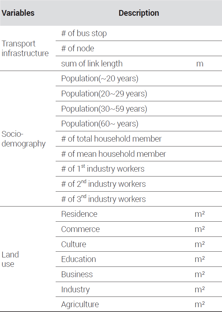
In this study, the origin-destination data between TAZs utilizes cell tower-based TAZs as the spatial units, which can be matched with targeted Si-gun-gu or eup-myeon-dong level data. This setup has the advantage of easily matching attribute information with cell tower-based TAZs if there is existing statistical data at the targeted Si-gun-gu or Eup-myeon-dong level. For the development of the trip generation model in this study, demographic variables related to population (Lafta and Ismael, 2022; Naser, 2020), socioeconomic indicators such as household size (Lafta and Ismael, 2022; Masoumi, 2022; Aboelenen et al., 2021; Usanga et al., 2020; Yang et al., 2020; Naser, 2020), transportation infrastructure variables including the number of bus stops, subway stations, and node-link density (Yang et al., 2020), and land use variables (Lee and Choo, 2021) were used as independent variables. The independent variables selected for this study are as shown in <Table 3>.

Table 3.

Selected Variables of trip generation models

4. Selection of analytical technique

For developing a trip generation model, the most commonly used analytical technique is linear regression analysis, such as multiple regression analysis (Takyi, 1990). However, the dependent variable in this study, trip production and attraction from mobile origin-destination data, does not meet the assumptions of normality and exhibits overdispersion, making a linear regression analysis unsuitable. Accordingly, this study has chosen the quasi-Poisson regression model as the analytical technique.

The quasi-Poisson regression model is one of the generalized regression techniques, and it is calculated as shown in Equation (1). Here, μ represents the mean of the dependent variable, x_j denotes individual independent variables, and β_j represents the regression coefficients. The quasi-Poisson regression model is more appropriate than the Poisson regression model for deriving regression models of overdispersed data (Gabriella et al., 2019).

Generalized regression models such as the quasi-Poisson regression model typically do not use the commonly used Adjusted R-Square for assessing model fit. Instead, values such as McFadden’s R-Square are used as the primary measure (McFadden, 1973). McFadden’s R-Square is derived as a scalar value between 0 and 1, where values closer to 1 indicate a better fit of the model. McFadden’s R-Square is calculated as shown in Equation (2), by subtracting from 1 the ratio of the log likelihood of the fitted model to the log likelihood of the null model.

1. Identification of key variables

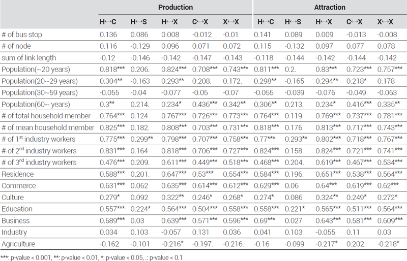
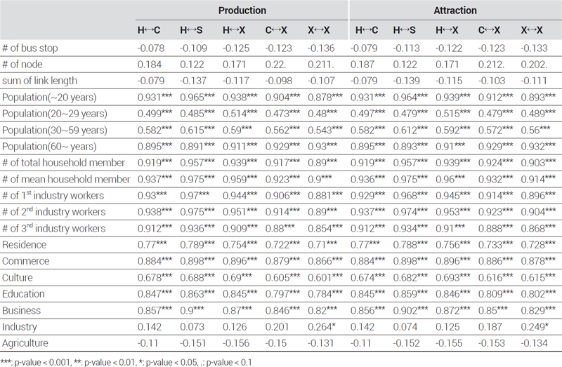
In this section, prior to developing city-specific trip generation models for different population sizes using mobile origin-destination data, a Pearson correlation coefficient analysis was conducted. The key variables selected for the trip generation model analysis had a significance level of p < 0.05 in correlation with the dependent variables, trip production and attraction. The results of the correlation analysis are presented in Tables 1, 2, 3, and 4 in the Appendix.

For the tourism city of Andong, significant correlations were found between PA-specific traffic volumes and several variables, including the sum of link length, number of total household members, number of mean household members, number of second industry workers, number of third industry workers, population under 20 years old, population in their 20s, population in their 30s to 50s, population over 60 years old, residential area, commercial area, cultural area, business area, and agricultural area. The variable for the number of nodes showed a positive correlation with non-household-based traffic volumes.

For the industrial city of Eumseong, significant correlations were found between PA-specific traffic volumes and variables such as number of total household members, number of second industry workers, number of third industry workers, population under 20 years old, population in their 20s, population in their 30s to 50s, population over 60 years old, residential area size, commercial area size, cultural area size, educational area size, and business area size. The number of mean household members showed a positive correlation with household-based commuting and other commuting trip volumes. Additionally, agricultural area size had a positive correlation with household-based other commuting traffic volumes. Household-based school commuting had significant correlations with only two variables: the number of second industry workers and educational area size.

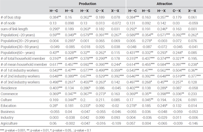
For the rural city of Euiseong, significant correlations were found between PA-specific traffic volumes and variables such as number of total household members, number of mean household members, number of first industry workers, number of second industry workers, number of third industry workers, population under 20 years old, population in their 20s, population in their 30s to 50s, population over 60 years old, residential area size, commercial area size, cultural area size, educational area size, and business area size. In the case of industrial area size, there was a positive correlation with non-household-based other traffic volumes.

For the fishing city of Sinan, significant correlations were found between PA-specific traffic volumes and variables such as the number of total household members, number of second industry workers, number of third industry workers, population under 20 years old, population in their 20s, population in their 30s to 50s, population over 60 years old, and commercial area size. The variables showing significant correlations varied slightly depending on the PA purpose.

2. Development of trip generation models by city function

in this section, a quasi-Poisson regression analysis is applied to derive the trip generation model, focusing only on variables that showed a significance level of less than 0.05 in the Pearson correlation analysis. To address the issue of multi-collinearity among the independent variables, the Variance Inflation Factor (VIF) values for all variables within the trip generation model were adjusted to be less than 5.

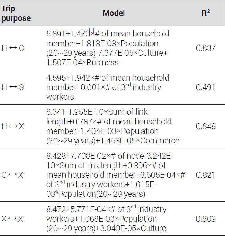
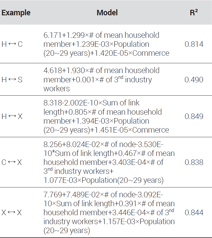
First, the results of developing PA-specific trip generation models for the tourism city Andong are shown in <Table 4> and <Table 5>. For household-based commuting, the production model included variables such as the number of mean household members, population in their 20s, cultural area size, and business area size, while the attraction model included the number of mean household members, population in their 20s, and commercial area size. For household-based school commuting, the production model included variables such as the number of mean household members and the number of third industry workers. The attraction model had the same variables.

Table 4.

The selected Andong-si trip production model

Table 5.

The selected Andong-si trip attraction model

For household-based other commuting, the production model included variables such as the sum of link length, number of mean household members, population in their 20s, and commercial area size. The attraction model had the same variables. For non-household-based work commuting, the production model included variables such as the number of nodes, sum of link length, number of mean household members, number of third industry workers, and population in their 20s. The same variables were used in the attraction model. For non-household-based other commuting, the production model included variables such as the number of third industry workers, population in their 20s, and cultural area size, while the attraction model included the number of nodes, sum of link length, number of mean household members, number of third industry workers, and population in their 20s.

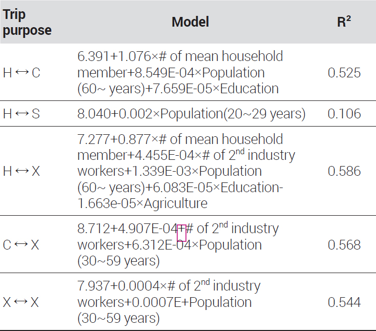
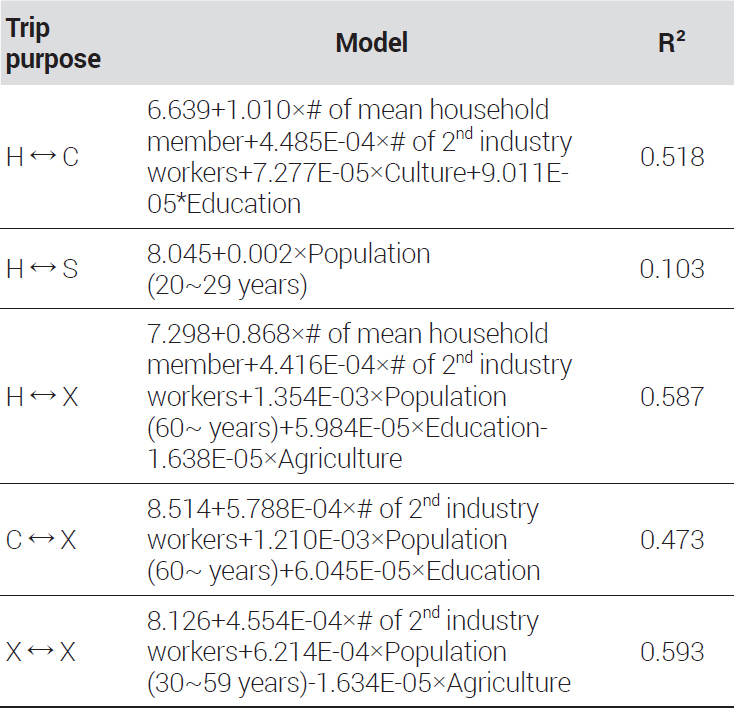
Second, the results of developing PA-specific trip generation models for the industrial city Eumseong are shown in <Table 6> and <Table 7>. For household-based commuting, the production model included variables such as the number of mean household members, number of secondary industry workers, population over 60 years old, and educational area size, while the attraction model included the number of mean household members, number of secondary industry workers, cultural area size, and educational area size. For household-based school commuting, the production model included variables such as population in their 20s, and the attraction model had the same variables. For household-based other commuting, the production model included variables such as the number of mean household members, number of secondary industry workers, population over 60 years old, educational area size, and agricultural area size. The attraction model had the same variables. For non-household-based work commuting, the production model included variables such as number of secondary industry workers and population in their 30s to 50s, while the attraction model included number of secondary industry workers, population over 60 years old, and educational area size. For non-household-based other commuting, the production model included variables such as number of secondary industry workers and population in their 30s to 50s, while the attraction model included number of secondary industry workers, population in their 30s to 50s, and agricultural area size.

Table 6.

The selected Eumseong-gun trip production model

Table 7.

The selected Eumseong-gun trip attraction model

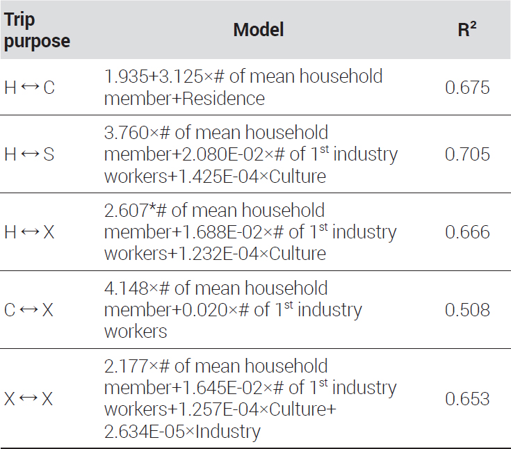
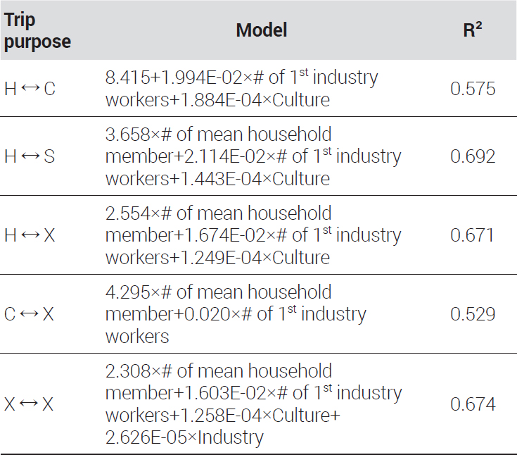
Third, the results of developing PA-specific trip generation models for the rural city Euiseong are shown in <Table 8> and <Table 9>. For household-based commuting, the production model included variables such as the number of mean household members and residential area size, while the attraction model included the number of first industry workers and cultural area size. For household-based school commuting, the production model included variables such as the number of mean household members, number of first industry workers, and cultural area size. The attraction model used the same variables. For household-based other commuting, the production model also included variables such as the number of mean household members, number of first industry workers, and cultural area size. The attraction model had the same variables. For non-household-based work commuting, the production model included variables such as the number of mean household members and number of first industry workers. The attraction model also used these variables. For non-household-based other commuting, the production model included variables such as the number of mean household members, number of first industry workers, cultural area size, and industrial area size. The attraction model had the same variables.

Table 8.

The selected Euiseong-gun trip production model

Table 9.

The selected Euiseong-gun trip production model

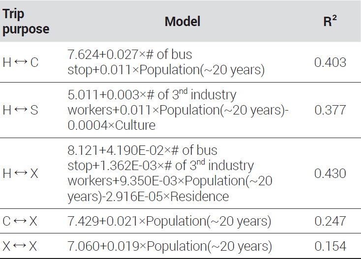
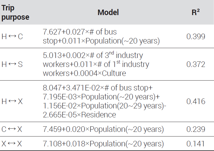
Fourth, the results of developing PA-specific trip generation models for the fishing city Sinan are shown in <Table 10> and <Table 11>. For household-based commuting, the production model included variables such as the number of bus stops and population under 20 years old. The attraction model used the same variables. For household-based school commuting, the production model included variables such as the number of third industry workers, population under 20 years old, and cultural area size, while the attraction model included the number of third industry workers, number of first industry workers, and cultural area size. For other household-based commuting, the production model included variables such as the number of bus stops, number of third industry workers, population under 20 years old, and residential area size, while the attraction model included the number of bus stops, population under 20 years old, population in their 20s, and residential area size. For non-household-based work commuting, both the production and attraction models included variables such as population in their 20s. Similarly, for non-household-based other commuting, both the production and attraction models included variables including population in their 20s.

Table 10.

The selected Sinan-gun trip production model

Table 11.

The selected Sinan-gun trip attraction model

3. Summary of analysis results

in the case of tourism cities, the main variables influencing traffic were identified as the number of mean household members, number of third industry workers, population in their 20s, and the sizes of cultural and commercial areas. For industrial cities, the primary variables included the number of mean household members, number of secondary industry workers, population over 30 years old, and educational area size. In rural cities, the key variables were the number of mean household members, number of first industry workers, and cultural area size. In fishing cities, the population under 30 years old was the only notable variable influencing travel.

The analysis results suggest that the variables influencing trip production and attraction vary depending on the function of the city. When conducting economic feasibility studies for road and railway projects, the area under influence is defined for estimating traffic demand, and this area usually covers multiple cities and counties. If the models developed in this study, which take into account city functions, are applied, more reliable trip generation values can be obtained.

However, in the case of tourism and industrial cities, the explanatory power of the models for household-based school commuting was found to be very low, between 0.1 and 0.2, compared to other models. When the explanatory power of a model is low, its utility for actual demand estimation is reduced, indicating a need to develop additional factors that can enhance the explanatory power.

Moreover, rural and fishing cities generally exhibited lower explanatory power in their models compared to other types of cities. This result may be due to the populations of rural and fishing areas being predominantly composed of older adults, leading to less active trip production and attraction. Indeed, the analysis of data from this study showed that mobile phone traffic participation among middle-aged and older populations in Sinan and Euiseong was higher than in Andong and Eumseong, as depicted in <Figure 2>. Conversely, the proportion of mobile phone traffic among the younger population, specifically those under 30, was higher in Andong and Eumseong.

Figure 2.

Trip proportion by age by city

In particular, the explanatory power of non-household-based commuting models in fishing cities was very low, below 0.3, suggesting that research on developing trip generation models for such cities should be conducted separately. Additionally, PA-based models, which reflect characteristics of both origin and destination TAZs, have shown challenges in incorporating land use or transportation infrastructure characteristics (Song et al., 2011). Therefore, to develop more refined PA-based trip generation models, it will be necessary to focus on incorporating a variety of socioeconomic indicators and demographic characteristics.