[ Article ]

Journal of Korea Planning Association - Vol. 56, No. 5, pp.239-255

ISSN: 1226-7147 (Print) 2383-9171 (Online)

Print publication date 31 Oct 2021
Final publication date 13 Aug 2021

Received 17 May 2021 Revised 13 Jul 2021 Reviewed 03 Aug 2021 Accepted 03 Aug 2021

DOI: https://doi.org/10.17208/jkpa.2021.10.56.5.239

Comparative Analysis of Energy Poverty Prediction Models Using Machine Learning Algorithms

Hong, Zhe^** ; Park, In Kwon^***

**Doctorate Candidate, Department of Environmental Planning, Seoul National University righttocity123@gmail.com
***Associate Professor, Department of Environmental Planning, Director of Environmental Planning Institute, Seoul National University parkik@snu.ac.kr

Correspondence to: ^*** Associate Professor, Department of Environmental Planning, Director of Environmental Planning Institute, Seoul National University (Corresponding Author: parkik@snu.ac.kr) This paper is a translation of a paper written in Korean into English, and a Korean version is released on the website(www.kpa1959.or.kr).

Abstract

The energy poor are vulnerable to energy costs, and their vulnerability is expected to increase with climate change. Therefore, accurately predicting energy poverty can help minimize damage cause by climate change to achieve social equity. This study aims to develop a series of models to predict energy poverty as well as analyze the relative importances and partial dependences of predictors by applying machine learning algorithms. Accordingly, we used the 2016 Household Income and Expenditure Survey data and applied different machine-learning methods, such as Decision Tree, Artificial Neural Network, Bagging, Random Forest, Extreme Gradient Boosting, and Support Vector Machine. The main results are as follows: First, the Random Forest model performs the best at predicting energy poverty. Second, household income, food expenses, living floor area, age of the householder, public transfer income, and educational attainment of the householder are the most important predictors. Third, using partial dependence plots (PDPs) and accumulated local effects (ALEs), we identified the nonlinear relationships between the six most important predictors and the response variable. Based on these findings, we expect to derive meaningful policy implications to identify the traits that affect the probability of a family’s energy poverty.

Keywords:

Energy Poverty, Prediction Models, Machine Learning Algorithms, Random Forest, Nonlinear Relationship

키워드:

에너지 빈곤, 예측모형, 머신러닝 알고리즘, 랜덤 포레스트, 비선형 관계

Ⅰ. Introduction

In modern society, people of all social classes should be able to afford a certain level of energy consumption. Those who are unable to consume the necessary amount of energy may undergo a decrease in physical functions, which may lead to severer health problems (Bouzarovski and Petrova, 2015). In the long term, the lack of sufficient heating and cooling due to energy poverty can cause diseases, such as chronic diseases, in the residents, and deteriorate the mental health by causing depression and stress (Lacroix and Chaton, 2015; Bosch et al., 2019). Therefore, more emphasis is put on the policies of energy welfare.

Starting from the UK, discussions on energy poverty have recently been reactivated in EU countries, including France and Spain (Hills, 2011, 2012; Romero et al., 2018). Many previous studies were conducted by using the TPR (Ten Percent Rule), proposed by Boardman (1991) as an indicator. However, as the TPR has a limitation that the high-income households that consume a large amount of energy may also be included in the energy-poor class, different multidimensional energy poverty indicators have been developed for a fresh new approach, including the LIHC (Low-Income High-Cost) by Hills (2011) and the MIS (Minimum Income Standard) by Moore (2012).

The major factors to energy poverty include the household characteristics, such as household income, household members, and elderly household; the householder characteristics, such as the householder age, gender, and education; the consumption characteristics, such as housing cost and food cost, and the residential characteristics including the dwelling area and homeownership (Healy and Clinch, 2004; Palmer et al., 2008; Maxim et al., 2017; Abbas et al., 2020; Legendre and Ricci, 2015).

While various studies have been conducted in Western countries including the UK, France, and Spain, few studies have been conducted in South Korea to analyze the factors to energy poverty. In addition, most of the previous studies were conducted by applying the traditional statistical techniques such as the logistic regression analysis, but few studies have been done to predict energy poverty by using machine learning algorithms.

With the recently increasing interest in the prediction of the targets of policies in the design of welfare policies, more and more studies about poverty are carried out by applying machine learning algorithms (Ajay et al., 2019; Verme, 2020). This is because machine learning algorithms are evaluated to have excellent performance in not only solving the policy prediction problems about ‘who’ should be the most appropriate targets of the policy but also exploring the nonlinear relations between the response variables and the predictor variables (Chalfinet al., 2016; Kleinberg et al., 2015).

In this context, the purpose of the present study is to apply machine learning algorithms that are suitable for the optimization of the prediction performance to develop a model for predicting the energy poverty in Korea and analyze the relative importance, the partial dependence plots (PDP) and the accumulated local effects (ALE) of the predictor variables. For this purpose, prediction models were developed by applying five machine learning algorithms, which are decision tree, bagging, random forest, extreme gradient boosting, and support vector machine, and the predictive power of the models was comprehensively evaluated to derive the optimal model.

The structure of this article is described below. Chapter 2 introduces the definition and measurement of energy poverty and reviews the previous studies about the factors to energy poverty. Chapter 3 describes the data used in this study as well as the variable measurement and the methodology. Chapter 4 presents the results of the comparison of the performance between the developed prediction models and discusses the importance and partial dependence of the predictive factors. Finally, Chapter 5 summarizes the analytical results and presents the policy implications.

Ⅱ. Theoretical Background and Previous Studies

1. Definition and measurement of energy poverty

The concept of energy poverty, initially emerging from the UK in the 1980s, has been discussed in various ways, but it is interchangeably used with the terms such as fuel poverty and energy burden. For example, fuel poverty is defined in the UK as ‘a household below the poverty line that needs to spend more than 10% of its income on fuel to use energy service of an appropriate level.’ In the US, the concept of energy burden is used on behalf of energy poverty. The energy burden is divided into home energy burden and residential energy burden; the former includes the energy cost for heating and cooling, and the latter includes the energy cost for not only heating and cooling but also the energy cost directly related to daily living, including the cost for lighting, hot water, and cooking.

Energy poverty can be measured in terms of objective indicators and subjective indicators. The objective indicators are objective items or standards that are used by a third party to measure energy poverty, including the household income and energy cost, while the subjects indicators are used to measure energy cost based on the subjective judgment on or the satisfaction with the energy cost that is necessary to maintain the basic living. The representative examples of the objective indicators are TPR (Ten Percent Rule), LIHC (Low Income High Cost), MIS (Minimum Income Standard), and CEPI (Compound Energy Poverty Indicator), and the examples of the subjective indicators are FFP (Feeling Fuel Poor) and PEP (Perceived Energy Poverty).

The TPR, the most popular indicator of energy poverty, was firstly proposed by Boardman in 1991. The TPR defines an energy-poor household as ‘a household of which necessary energy expenditure is 10% or higher than the income.’ The household income means the disposable income, and the necessary energy expenditure means the cost of fuel that needs to be spent to maintain a certain range of temperature (18-21℃ for heating and cooling). The cost of fuel is not the actual expenditure for fuel but is estimated as the value obtained by multiplying the theoretical fuel consumption by the average energy price. The TPR can be easily calculated, but it has a limitation that the high-income class having a high energy consumption level may also be included in the energy-poor class (Hills, 2011).

To overcome the limitation of the TPR that it cannot clearly distinguish income poverty from energy poverty, Hills (2011; 2012) proposed the LIHC. The LIHC considers as an energy-poor household ‘a household of which the household income, except the fuel cost and residential cost, is below the poverty line (below 60% of the median income), and of which energy expenditure is higher than the median value of all households.’ The LIHC seems to be useful in that it reflects the criteria related to not only the income but also the energy expenditure. However, LIHC has the problem that a household of which fuel expenditure is lower than the criterion may be excluded from the energy-poor class, even if its actual income level is very low.

Considering the problem, Moore (2012) proposed the MIS, focusing on the capability of households to pay the energy expenditure. The MIS defines an energy poor household as ‘a household of which necessary fuel expenditure is higher than the amount obtained by subtracting the necessary residential cost and the minimum living cost from its income.’ The minimum living cost refers to the minimum cost of acceptable living according to the household type and the residential area. The MIS is significant because the fuel cost is calculated in consideration of the minimum cost of living, unlike the TPR and LIHC. The MIS is difficult to calculate objectively by applying the same standards because the minimum cost of living is significantly dependent upon the social context and the institutional background of different countries.

Aguilar et al. (2019) develop the CEPI to reflect both the low income and the low fuel expenditure. The CEPI defines an energy poor household as ‘a household of which disposable income is below the poverty line (below 60% of the median income), and of which energy expenditure is higher than both the median value of all households and 10% of its income.’ The CEPI can compensate for the limitations of the TPR and LIHC to capture the characteristics of energy poverty, but it fails to reflect the characteristics and energy efficiency of the residential space.

In contrast to the objective indicators, the subjective indicators are used to measure energy poverty through the subjective evaluation of the self-satisfaction with the energy consumption, considering that individual households have different levels of necessary energy consumption. Price et al. (2012) discussed the FFP, a subjective energy poverty indicator, by using the data from the Family Expenditure Survey for UK Households. Meyer et al. (2018) employed a subjective indicator called PEP to investigate energy poverty by using the data from a survey conducted in Europe. The PEP, proposed by Meyer et al. (2018), is focused on the capabilities of households to pay the actual energy expenditure and the level of recognition. The PEP indicator measures energy poverty from two perspectives: if the energy expenditure is burdensome to the household, and if the household is capable of paying the energy expenditure for the heating and cooling of the house to maintain an appropriate temperature.

In Korea, various approaches have been made to define and measure energy poverty. For example, Kim (2015) employed a hybrid-type indicator, defining an energy poor household as ‘a household incapable of maintaining an appropriate level of heating or a low-income household of which the fuel expenditure accounts for 10% or more of the current income.’

Jin et al. (2010), dividing energy poverty into absolute poverty and relative poverty, defined an absolute poor household as ‘a low-income household in the bottom 30% income bracket of which energy consumption is below the minimum lightning and heating expense,’ and a relative poor household as ‘a low-income household of which energy expense exceeds 11.5% of the disposable income.’ Similarly, Oh and Jin (2021) defined energy poverty as ‘a state of feeling burdened to pay the expense of energy that is necessary to keep an appropriate level of living,’ and divided it into absolute energy poverty measured as ‘the ratio of the actually paid lightning and heating expense to the minimum lightning and heating expense’ and relative energy poverty measured as ‘the ratio of energy expense to the income.’

Lee (2019) defined an energy-poor household as ‘a household in a state of being unable to use the needed energy at an appropriate level due to an economic reason,’ and identified energy-poor households by surveying ‘whether the household has experienced discontinuation of the electricity, telephone or water supply or failed to afford heating in cold winter for being unable to pay at least one of the electric bill, phone bill and water bill for lacking money.’

2. Factors to energy poverty

The major factors to energy poverty are a high energy price, a low-income level and, a low energy efficiency (Palmer et al., 2008; Maxim et al., 2017). A rise in the energy price reduces the affordable energy resources and increases the burden of energy expense, resulting in more energy-poor households. In the UK, for example, the increase of the energy price by 1% increased the energy-poor households by about 0.05% (City of Liverpool, 2007). The energy price is also related to energy accessibility. The energy expense was found to be higher in the areas where low-income households are concentrated or in the rural areas due to the lack of accessibility to low-price energy sources (Crentsil et al., 2019; Tod et al., 2012). In the low-income areas or rural areas, the households have no choice but to utilize relatively expensive fuels such as coals and LPG, because the urban gas, which is cheap and safe, is not available there.

On the other hand, low-income households having economic difficulties are more likely to be energy-poor households (Abbas et al., 2020; Healy and Clinch, 2004; Romero et al., 2018). A low-income household, which may not afford the necessary energy, can easily become an energy-poor household. The energy inefficiency is related to the housing quality; an older house often has insufficient insulation facilities or a poor residential environment, and thus causes energy waste, which leads to an increase of the energy expense (Bouzarovski and Petrova, 2015; Legendre and Ricci, 2015; Masuma, 2013).

The sociodemographic characteristics of the householder, including age, education, gender, and marital status, also affect energy poverty; a household where the householder is a woman, low in age and educational level, and lives alone is more vulnerable to energy poverty (Abbas et al., 2020; Healy and Clinch, 2004; Legendre and Ricci, 2015; Romero et al., 2018). This is because a householder who is older and has a higher educational level utilizes energy more efficiently and has more experience and knowledge about the household consumption expenditure appropriate for the household income. In addition, a female householder has a lower household income level and a lower residential level and is more sensitive to the temperature change, and thus is more likely to be included in the energy poverty class, compared with a male householder (Abbas et al., 2020; Kaikaew et al., 2018).

The household characteristics, such as a single-person household, a household with a child, and a household with a disabled person, also affect energy poverty (Healy and Clinch, 2004; Legendre and Ricci, 2015). In particular, a household where there is a household member who is disabled or a child under age is more likely to be in energy poverty (Masuma, 2013; Romero et al., 2018). This is basically because the people in a socially vulnerable class, such as children and the disabled, often have a lower income level, as they have fewer opportunities to participate in the economic activities, and they spend more energy to keep an appropriate temperature and thus have more energy burden, as they stay longer in the houses and are more sensitive to the temperature change (Kousis et al., 2020; Snell et al., 2015; Healy and Clinch, 2004).

Besides, other items of living expenses for food, healthcare and residence are also closely related to energy poverty, because they affect the energy consumption pattern of low-income households (Dubois, 2012; Sovacool, 2015). This is because the money that can be spent on energy is decreased in the low-income households that spend much on residence and food. As a result, such households are more likely to be included in the energy poverty class, as they are affected by the economic difficulties more seriously.

In addition, residential characteristics, including dwelling area, type of housing, and type of occupancy, also affect energy poverty. Although the dwelling area is an important factor of energy poverty, the results are not consistent. For example, a study conducted in the UK (Masuma, 2013) showed that the vulnerability to energy poverty was greatly increased when the dwelling area was over 50 m², but a study conducted in several East Asian countries (Abbas et al., 2020) showed that the energy poverty level was decreased as the dwelling area was increased. In general, detached houses are more vulnerable to energy poverty than apartments (Masuma, 2013). In addition, renting households were found to be more vulnerable to energy poverty because of the higher hosing cost and the lower energy efficiency of the houses (Kousis et al., 2020; Legendre and Ricci, 2015; Romero et al., 2018).

3. Previous studies on energy poverty

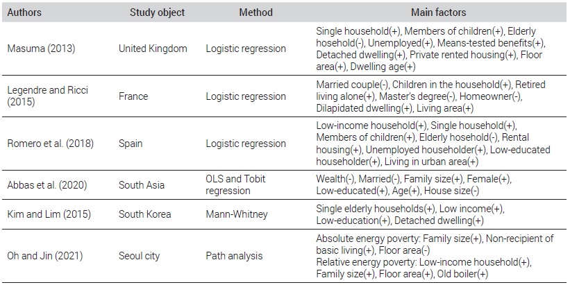
With the increasing interest in the issue of energy poverty, many studies have been conducted on energy poverty in Korea and other countries (see Table 1). With regard to the overseas studies, Masuma (2013) performed a logistic regression analysis with the energy-poor households in the UK and reported that single-person households, households with children under age, unemployed householders, detached houses, private rental houses, wide dwelling areas, and old houses are positively correlated with the probability to be predicted as an energy-poor household.

Table 1.

Summary of selected previous study on factors of energy poverty

Legendre and Ricci (2015) employed a logistic regression model to investigate the energy poverty in France, and showed that people who live together with a spouse, who have a high education level (master’s degree or higher), and who are home-owners are less vulnerable to energy poverty, while those who are a retired senior who live alone or those who live in an old house or have a wide dwelling area are more likely to be included in the energy poverty class.

Romero et al. (2018) performed a logistic regression analysis in Spain and found that single-person households, households with children under age, rental houses, unemployed householders, low-income households, householders with a low education level, and urban households are move vulnerable to energy poverty.

Abbas et al. (2020) analyzed the factors to energy poverty by applying the Tobit model to 674,834 households in East Asian countries and reported that wealth, being married and a large house size decrease the level of energy poverty, while a large family size, a female householder, a low educational level, and an old age increase the level of energy poverty.

Most of the studies conducted in Korea are focused on the analysis of the characteristics of energy consumption and energy poverty, and few studies have been conducted to directly deal with the factors to energy poverty. Kim and Lim (2015) performed a Mann-Whitney nonparametric test with regard to the energy consumption and energy poverty of the households with an elderly member and the households without an elderly member by using the data from the 2014 Monthly Household Income and Expenditure Survey and reported that the ratio of the fuel expense to the income was highest in the households of a single elderly person, and was significantly higher in the households with a householder having a low educational level and the households in detached houses.

Oh and Jin (2021) performed a path analysis with respect to energy consumption and poverty characteristics with the low-income households in Seoul and showed that the number of household members, housing type, dwelling area, and beneficiary of the basic living subsidies have a significant effect on the energy consumption and poverty characteristics. Specifically, the absolute level of energy poverty was higher in the households with many household members, those whose householders are not a beneficiary of the basic living subsidies, and those with a smaller dwelling area. In addition, the relative energy poverty level was higher in the households with a lower income level, those with many members, those with a wider dwelling area, and those with a low heater efficiency.

4. Differences from previous studies

Compared with the previous studies reviewed earlier, the present study has the differences described below. First, the subjects of the study are different. Most of the present studies were conducted in the Western countries, including the UK, France, and Spain, and only several studies have been conducted in Korea to analyze the factors to energy poverty. The previous studies conducted in Korea are mostly focused on the analysis of the factors to the energy consumption or the estimation of the size of the energy poverty class. Korea may show a pattern of energy poverty that is different from that of Western advanced countries, because of the residential culture centered on apartments and the high density of the urban areas. Therefore, analyzing the factors to energy poverty in Korea is significant in evaluating the applicability of the overseas studies and the uniqueness of Korea.

Second, the research method is different. Most of the previous studies were conducted by employing the traditional statistical techniques such as logistic regression analysis, but the studies conducted to predict the energy poverty class by using the machine learning techniques are very few. Most of the conventional statistical models assume that the relations between the explanatory variables and the dependent variables are linear or quadratic, thus lacking suitability to atypical relations and having limitations in accurately classifying and predicting dependent variables (Géron, 2019). The machine learning-based prediction models allow for flexibly handling atypical relations between variables and show much higher predictive power. However, the machine learning techniques also have limitations, because the prediction process is hard to understand accurately, and the statistical significance of the independent variables is difficult to verify. Despite these limitations, considering that the accurate and rapid identification of the policy targets is gaining more importance in policy enforcement, and thus the prediction models are required to show higher predictive power. Therefore, the application of machine learning algorithms is important in predicting energy poverty. In addition, the present study is meaningful in that the results were compared between the traditional logistic models and the machine learning models based on various algorithms in order to evaluate the predictive power.

Ⅲ. Study Design

1. Subjects of study and measurement of variables

The present study was conducted to predict energy poverty by using the 2016 Household Income and Expenditure Survey. The Household Income and Expenditure Survey, conducted by the National Statistical Office, is one of the long-standing cross-sectional surveys that have nation-wide representativeness. This survey is conducted each month with the sample households in the entire country by investigating the information related to the household income and expenditure in order to understand the change of the income and consumption level of the citizens.

In this study, the annual data from the survey was used instead of the monthly data in order to control the seasonality of energy consumption by households (Sharma and Kumar, 2019). In addition, rather than the data for the latest year, the data for 2016 was used, because the accurate household income was difficult to find from the annual data for 2017, as the survey item about household income was changed from the previous question asking the specific amount to the new question asking the income quintile bracket. The annual raw data of the 2016 Household Income and Expenditure Survey included the survey results from 8,947 households. The data that was finally used in the present study for the analysis included the results from 8,510 households, as the missing values of the household income or energy consumption and some outliers (0.5% of all samples) of the dwelling area, housing cost, and healthcare cost were excluded from the dataset.

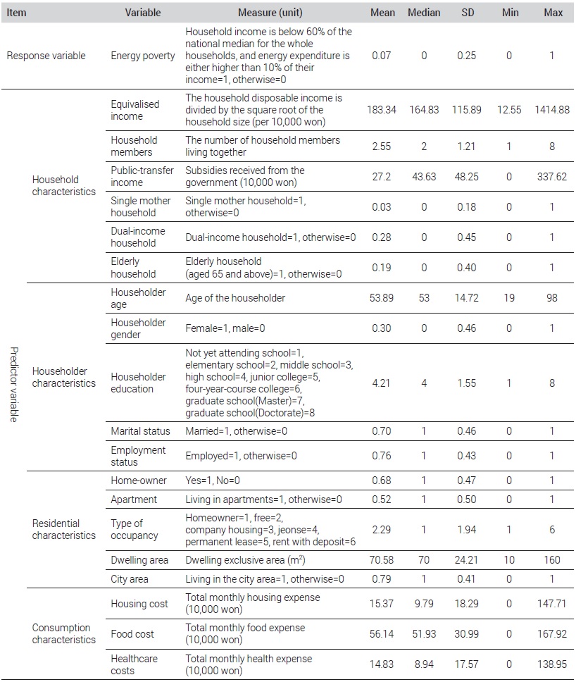
Table 2 shows the variable measurement and the descriptive statistics. Energy poverty, the response variable, was defined with reference to the CEPI indicator proposed by Aguilar et al. (2019) as a household of which income is below the official public line (60% of the national median income) and of which the ratio of the fuel expenditure to the average monthly income is 10% or higher. The CEPI indicator was referred to, because it is a recently proposed measurement indicator that can reflect both the low-income level and the low fuel expense of energy-poor households, overcoming the limitations of the conventional TPR and LIHC indicators. In particular, the fuel expense, referring to the cost of fuel spent on daily housework, including lightning, heating, cooling, and cooking, includes the expense for electricity, city gas, heating, and fuels, including Diesel. The monthly average fuel expense of the sample households was about 88,900 KRW (median: 80,500 KRW) with a maximum of 667,600 KRW and a minimum of 0 KRW.

Table 2.

Variable measurement and descriptive statistics

The predictor variables consisted of household characteristics, householder characteristics, residential characteristics, and consumption characteristics. Specifically, the household characteristics included the variables of household income, household size, public-transfer members, single-mother household, dual-income household, and elderly household. The household income was measured as the equivalized disposable income in consideration of the number of household members living together. The household size was measured as the number of household members living together. The public-transfer income included the government subsidies, including public pension, unemployment benefits, and housing benefits. The single-mother household was defined as a household consisting of a female householder and a child under the age of 18 years. The dual-income household was defined as a household in which the couple (householder and the spouse) are both employed whether they live together or not. Finally, the elderly household was defined as a household including a household member who is at the age of 65 years or older.

The householder characteristics included age, gender, education, marital status, and employment status. The householder gender was set to be female in the default setting. The default setting for education was ‘Not yet attending school,’ and other options included an elementary school, middle school, high school, junior college, fouryear-course college, graduate school (master), and graduate school (doctorate). The default marital status was ‘Married.’ The employment status was about the employment of the householder.

The residential characteristics consisted of home-owner, apartment, type of occupancy, dwelling area, and city area. The consumption characteristics consisted of the housing cost, food cost, and healthcare cost.

2. Machine learning algorithms

1) Decision tree

The decision tree is an algorithm where tree-like structures connected with nodes are formed to find out through learning the patterns or rules included in the data and preparing them as models to perform classification and prediction (Breiman et al., 1984). The decision tree algorithm consists of steps of growing, pruning, validation, and prediction and interpretation. In the growing stage, considering the data structure and purpose of the analysis, appropriate splitting criteria and stopping rules that determine the time for expanding the nodes are designated to form a tree structure. In the pruning step, the branches that may cause an overfitting issue are removed. In the validation stage, the decision tree is evaluated by using a risk chart, profit chart, or cross-validation with test data. In the final stage of prediction and interpretation, the established tree model is finally predicted and interpreted.

The splitting criterion is purity or impurity which represents the degree of distribution of the target variable. A splitting variable that maximizes the sum of purity or one that minimizes the sum of impurity is finally selected as the splitting criterion. The impurity indexes of the decision tree include classification error, the Gini index, and the entropy index.

2) Bagging

Bagging, an abbreviation of bootstrap aggregating, is an algorithm for an ensemble learning-based model. In this algorithm, n datasets are generated from a single piece of training data through bootstrap re-sampling, and the individual datasets are aggregated to make n models for the voting of the final model based on the mean predictive values of the models (Breiman, 1996). Ensemble learning is a technique to generate several single learners and combine the prediction results from the learners in order to derive a more accurate learner. Bagging generally shows good prediction performance in an unbiased and stable model. Therefore, the growing of the tree is set to be the maximum, and pruning is skipped in many cases where bagging is applied.

3) Random forest

Random forest is an algorithm for an ensemble learning-based model, and it combines many decision trees through the basic principles of bagging and the bootstrap method (Breiman, 2001). In particular, in the random forest algorithm, the samples and the predictor variables are randomly set up through bootstrapping to repeatedly constitute independent decision trees and thereby reduce the prediction errors. Since a greater number of decision trees allows for the establishment of a more stable and accurate model, the random forest algorithm can increase the prediction power of a model by overcoming the limitations of a single decision tree or bagging, such as the low stability and accuracy and the overfitting issue. In the random forest algorithm, the model performance is evaluated by using Out-of-bag (OOB), which refers to the data that is not extracted in the bootstrap sampling and is used in behalf of a test set. The random forest algorithm can provide the OOB error.

The random forest algorithm can use the predicted error rate for classification or the Gini index to provide the relative importance of the predictor variables in two different ways. The first is to calculate the mean decrease accuracy (MDA). The basic idea is to calculate the error rate for classification (or accuracy) in random trees generated each time, calculate the error rate for classification again after excluding specific predictor variables, and then compare the two calculation results. If the excluded variable is not significant, there will be no significant difference between the two calculation results. A standardized MDA of the predictor variables is obtained by repeatedly performing the calculation process. A higher MDA means higher importance of the predictor variable. The second is to calculate the mean decrease Gini (MDG) based on the mean decrement of the Gini index when a predictor variable is divided from all random trees. The higher the importance of the predictor variable, the more decrement of the Gini index by the division. However, the MDA is used more often in practice, because the MDG is biased and has been known to fails to provide robust results (Sandri and Zuccolotto, 2010).

On the other hand, the random forest algorithm provides partial dependence upon the predictor variables, which represents the average marginal effect of the predictor variables on the response variable (Friedman, 2001; Liaw and Wiener, 2002). The partial dependence upon an individual predictor variable is to investigate the detailed relationships between the predictor and the response variable by calculating the prediction probability of the response variable while controlling for the average effects of the other predictor variables (Greenwell, 2017: 422).¹⁾ However, since the analysis of the partial dependence plots (PDP) may be biased when the correlations between the predictors are high, various other methods have recently been proposed as alternatives, including Individual Conditional Expectation (ICE), SHapley Additive exPlanations (SHAP), and Accumulated Local Effects (ALE) (Molnar, 2020). In particular, the ALE analysis is considered more unbiased, because the average effects of the predictor variables on the response variable may be understood, and the analytical results are unaffected by the correlations of the predictor variables (Molnar, 2020).

4) Extreme gradient boosting

XGBoost, the abbreviation of Extreme Gradient Boosting, is an algorithm upgraded from the existing Gradient Boosting Machine (GBM) (Chen and Guestrin, 2016). XGBoost also employs the decision tree as a boosting method, like the GBM, but the learning or classification speed, based on parallel processing, is much faster than that of the GBM. In addition, the prediction model has robustness due to the overfitting regularization, and the built-in cross-validation function makes the verification easy. Boosting refers to the method to sequentially train weak learners, and give weight to erroneously predicted data to improve the error in order to produce strong learners.

5) Support vector machine

The Support Vector Machine, proposed by Vapnik and his colleagues, is a machine learning algorithm to find out a hyperplane in a higher-dimensional space to perform classification or regression (Boser et al., 1992). The Support Vector Machine generally obtains a hyperplane that best classifies the data to classify the data into groups of similar values, and the hyperplane has a boundary surface where the margin of the individual groups is the maximum. The margin means the distance from the hyperplane that distinguishes the classes to training data near to the hyperplane. The training data positions at the hyperplane are called support vectors. Generally, the boundary of a support vector machine has a linear hyperplane when the boundary can be divided linearly. In a nonlinear case, the hyperplane is found by using slack variables and applying a radial basis function kernel that allows a measure of classification errors.

6) Artificial neural network

The Artificial Neural Network (ANN), a part of the artificial intelligence theory, is a model that is realized by imitating through a computer the information processing in the human brain, such as information transfer, decision-making, and learning (McCulloch and Pitts, 1943; Rosenblatt, 1958). The ANN basically consists of an input layer, a hidden layer, and an output layer, each of which has at least one node (or neuron). In particular, the nodes in each layer are connected with the nodes in another layer through weight. In the training process, the training data given to the input layer are summed up according to the weight, converted into an activation function in the hidden layer, and then transferred to the output layer.

Generally, the ANN employs a feed-forward or back-propagation method. In the feed-forward method, the operation of the given training data is performed in the forward direction from the input layer to the output layer. In the back-propagation method, the errors are firstly estimated with respect to the training data, and modified in the opposite direction from the output layer to the input layer (Rumelhart et al., 1986).

3. Performance evaluation method and analysis process

In the present study, a confusion matrix was used to evaluate the performance of the prediction model established by machine learning. Confusion matrices are classified into four categories: TP (True Positive), TN (True Negative), FP (False Positive), and FN (False Negative). TP refers to the case where the actual observation and the prediction are both positive; TN refers to the case where the actual observation and the prediction are both negative; FP refers to the case where the actual observation is negative but the prediction is positive; and FN refers to the case where the actual observation is positive but the prediction is negative.

In a study conducted by machine learning, a confusion matrix is used to provide the probabilistic performance evaluation indexes, such as accuracy, specificity, precision, recall, and F1-score. The accuracy refers to the ratio of correctly predicted observations to the total observations; the specificity refers to the ratio of correctly predicted negative observations to the total actual negative observations; the precision refers to the ratio of correctly predicted positive observations to the total predicted positive observations; the recall refers to the ratio of correctly predicted positive observations to the total actual positive observations; and the F1-score refers to the harmonic mean of the precision and the recall.²⁾

The present study was conducted by using the data from the 2016 Monthly Household Income and Expenditure Survey with a total of 8,814 observations from the samples. To evaluate the performance of the prediction model, 70% of the data was randomly allocated to a training dataset, and the remaining 30% to a test dataset. Next, to prevent the overfitting issue and find the optimal parameters in the data training process, the hyper-parameters of the prediction model were verified through 3-repeated 10-fold cross-validation. In other words, the original training data were randomly split into 10 new training data and validation data, and the resulting 10 evaluation data were used three times repeatedly to conduct the performance validation process. The optimal prediction model was derived by using the performance evaluation indexes, such as accuracy, specificity, recall, precision, and F1-score. Based on the final prediction model, the relative importance of the predictor variables and the detailed relations with the response variable were investigated by analyzing the PDP and ALE.

Ⅳ. Analytical Results

1. Establishment of the optimal prediction model

The accuracy of learning is generally increased in machine learning, as the epochs are increased. However, the increase of the epochs may cause an overfitting issue. To prevent overfitting, early stopping or K-fold cross-validation is usually carried out. In this study, 3-repeated 10-fold cross-validation was performed to establish an optimal prediction model.

1) ANN

The ANN model employed in this study is a simple prediction model consisting of an input layer, a hidden layer, and an output layer. Specifically, the mean accuracy was performed through cross-validation by setting the hidden unit to 1, 3 and 5 and the weight decay to 0, 0.0001, and 0.1. According to the test results, a model having a weight decay of 0.1 and a single hidden unit showed the highest accuracy of 0.9377, and thus was derived as the optimal model.

2) Decision tree

In the decision tree algorithm, a complexity parameter is generally used in the pruning stage to prevent the overfitting issue by controlling the tree size. The complexity parameter, which is a weight combining the error rate for classification and the leaf node, is used to control the complexity of the tree. In this study, the complexity parameter was set to be 0.0208, 0.0718, and 0.0868 for each cross validation to calculate the average accuracy. The analytical results showed that the accuracy of the decision tree model was 0.9411, which was the highest, when the complexity parameter was 0.0208.

3) Random forest

In the random forest algorithm for an ensemble learning model, it is critical to appropriately determine the number of trees (ntree) and the number (mtry) of the predictor variables that are used to split the tree nodes. The model performance is generally increased, as the number of trees is increased.

In the present study, the number of the predictor variables used in the tree node splitting was set to be 2, 10, and 10, and the number of the trees was increased from 300 to 800 to calculate the average accuracy through cross-validation. The analytical results showed that the model accuracy was highest at 0.9514 when the number of the used predictor variables was 10 and the number of the tress was 500, and thus the model was selected as the optimal model.

4) Extreme gradient boosting

In XGBoost, hyper-parameter tuning is necessary to prevent overfitting and derive an optimal prediction model. In this study, the learning rate was set to 0.3 and 0.4, the number of times of tree repetition and boosting (nrounds) 1, 2, and 3, and the maximum tree depth (max_depth) to 1, 2, and 3. In addition, the ratio of the predictor variables used in the tree generation was set to 0.6 and 0.8, and the ratio of the random samples used in the tree generation to 0.5, 0.75, and 1 to perform cross-validation and calculate the accuracy of the prediction model. The analytical results showed that model accuracy was highest as 0.9502 when the learning rate was 0.3, the number of times of tree repetition and boosting was 50, the maximum tree depth was 3, the ratio of the predictor variables used in the tree generation was 0.8, and the number of the random samples was 1. Therefore, the model was selected as the optimal XGBoost model.

5) Support vector machine

In the support vector machine, the radial basis function (RBF) kernel is generally used to predict the nonlinear characteristics vector. In particular, the improvement of the prediction performance of an RBF-based model requires the optimal combination of the cost parameter, which controls the penalty for the classification error, and the sigma value, which controls the nonlinearity of the kernel function.

In the present study, the cost parameter was set to 0.25, 0.5, and 1, and the sigma to 0.0211, 0.0302, and 0.0405 to calculate the average accuracy through cross-validation. The support vector machine having a cost parameter of 1 and a sigma of 0.0405 showed the highest accuracy of 0.931 and thus was selected as the optimal model.

2. Performance evaluation results of prediction models

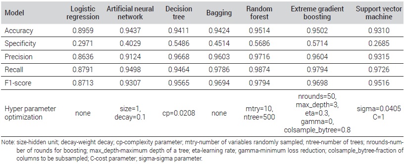
In the present study, models for predicting the energy poverty class were established by using the traditional logistic, ANN, decision tree, bagging, random forest, EGBoost, and support vector machine algorithms, and their prediction performance was compared. As shown in Table 3, the accuracy, representing the performance of the prediction models, was 89.59% in the logistic model, 94.37% in the ANN model, 94.11% in the decision tree model, 94.24% in the bagging model, 95.14% in the random forest model, 95.02% in the EGBoost model, and 93.10% in the support vector machine model, indicating that the accuracy was highest in the random forest model. This means that the ratio of the number of correctly predicted households to the total number of the subject households was highest in the random forest model. The specificity was much lower than the accuracy in all the models, but the XGBoost model showed the highest specificity among all the prediction models.

Table 3.

Performance evaluation of machine learning models

The recall, referring to the ratio of predicting the actual energy-poor households as an energy-poor household, was highest in the random forest model (97.16%). The precision, referring to the ratio of the actual energy-poor households to the household predicted as an energy-poor household, was also highest in the random forest model (98.74%). The F1-score, considering both the recall and the precision, was also highest in the random forest model (97.94%).

Summarizing the test results described above, the random forest model was found to be the best in the overall prediction of energy poverty with respect to 4 evaluation indexes out of 5. Therefore, the random forest model was selected as the final model and analyzed in terms of relative importance, partial dependence, and ALE.

3. Relative importance

The effects of the predictor variables are generally difficult to analyze in a model based on machine learning, but the relative importance of the predictor variables may be investigated in a random forest model. While the traditional statistical models provide an absolute measure, the statistical significance of the predictor variables, only the relative importance of the variables can be found in machine learning-based models. Nevertheless, the relative importance helps to identify the variables that should be firstly taken into consideration when the prediction is performed from limited data. Figure 1 shows the relative importance of the predictor variables of energy poverty with reference to the MDA. The top 10 predictor variables in terms of relative importance were household income, food expense, living floor area, householder age, public-transfer income, householder education, household size, elderly household, dual-income household, and type of employment. Although not shown here, these variables were all verified in the logistic regression model as significant variables within a significant level of 10%. The key analytical findings are described below.

Figure 1.

Variable importance plot (MDA)

First, 5 out of the top 10 predictor variables in the relative importance were related with the household characteristics, which are household income, public-transfer income, dual-income household, household size, and elderly household. Notably, the relative importance of household income (133.58) was much higher than that of other predictor variables, suggesting that household income is the most important factor in the prediction of energy-poor households.

Second, among the household characteristics, public-transfer income was found to be the 5^th important predictor variable, which means that public assistance from the government is an important factor in relieving the economic burden of the energy-poor households.

Third, among the residential characteristics, the living floor area showed high prediction power in predicting energy poverty. This suggests that the living floor area is an important factor in the prediction of energy poverty.

Fourth, the relative importance of food expense, a consumption characteristic, was higher than that of householder age and householder education. This shows that food expense is more important than the demographic variables about householders in the prediction of energy-poor households.

4. Partial dependence and accumulated local effects

The previous section of this article provides the importance of the predictor variables of energy poverty, but how the predictor variables are related to energy poverty is not identified. The random forest model allows for flexibly exploring the relationships between the predictor variables and the response variable because the relations are not assumed to be linear.

Figure 2 shows the partial dependence of the top 6 important predictor variables, which are household income, living floor area, food expense, public-transfer income, householder age, and householder education. The partial dependence represents the average marginal effect with respect to the probability of being predicted as energy poverty depending on the change of the predictor variables. The key findings are described below.

Figure 2.

Partial dependence plots

First, the probability of being predicted as energy poverty was increased, as the household income, one of the household characteristics, was increased by one unit. However, the probability of being predicted as energy poverty was drastically decreased, as the household income was increased over 1,470,000 KRW. As of 2016, the minimum cost of living for 3-person households was about 1,430,000 KRW, which was similar to the boundary value derived in the present study. This suggests that the probability of being an energy-poor household may be drastically increased, as the household income is decreased below the minimum cost of living.

Second, the probability of being predicted as energy poverty was continuously increased, as the living floor area, one of the residential characteristics, was increased by one unit. However, the probability of being predicted as energy poverty was considerably decreased, as the living floor area was increased over about 60 m². Since the houses smaller than 60 m² are commonly classified as small houses, these results show that the probability of being predicted as energy poverty is very high among small houses.

Third, the probability of being predicted as energy poverty was continuously increased, as the food expense, one of the consumption characteristics, was increased by one unit. However, the probability of being predicted as energy poverty was gradually decreased, as the food expense was higher than about 470,000 KRW, which is similar to the average food expense of low-income households calculated from the 2016 Korea Welfare Panel Study data (420,000 KRW). This means that the probability of being predicted as energy poverty is very high among households where the food expense is less than 470,000 KRW.

Fourth, the probability of being predicted as energy poverty was not significantly dependent upon the householder age, one of the householder characteristics, in the range from their 20s to late 50s, but it was significantly decreased from early 60s. Householders in their 60s usually retire from economic activities and their children start to form separate families. The probability of energy poverty may be decreased from the householder age of 60s, probably due to the retirement of the householders and the family separation of their children, which results in a decrease in energy consumption.

Fifth, the probability of being predicted as energy poverty was continuously decreased, as the public-transfer income, one of the household characteristics, was increased by one unit. The probability of energy poverty was drastically decreased, as the public-transfer income was increased over 1,320,000 KRW. However, the households that receive this amount of public-transfer income correspond to the top 4.78% of all the households, and thus the number is very small.

Sixth, the probability of being predicted as energy poverty was increased, as the householder education, which is one of the householder characteristics, was increased. However, when the householder education was elevated from high school graduation, the probability of being predicted as energy poverty was continuously decreased. Therefore, the plot had an inverse U-shape. This may be because when the householder education is low, the income level is generally low but the energy consumption is increased (Legendre and Ricci, 2015).

Through the PDP analysis, the random forest model allowed for exploring the nonlinear relations between the predictor variables and the response variable, which are difficult to investigate through the conventional linear model. However, an alternative is needed, because the PDP analysis may be biased when the predictor variables are highly correlated. Therefore, an ALE analysis was performed in this study to examine if the PDP analysis is robust. The results of the ALE analysis showed patterns that are very similar to the PDP analysis. This means that the results of the PDP analysis were robust without being severely biased. This suggests that the results from the PDP analysis are similar to the results from the ALE analysis when the predictor variables used in the model are not highly correlated.

Ⅴ. Conclusions

The present study was conducted by using the data from the 2016 Monthly Household Income and Expenditure Survey to develop models for predicting energy poverty by applying machine learning algorithms and analyze the importance and partial dependence of predictor variables. The key analytical results are described below. First, the random forest model showed better performance than other prediction models in predicting energy poverty. Second, the analysis of the relative importance of the predictor variables showed that household income, living floor area, food expense, householder age, public-transfer income, and householder education have importance in the prediction of energy-poor households. Third, the PDP and ALE analyses verified the nonlinear relations between the predictor variables and the response variable. Specifically, the probability of being predicted as energy poverty was decreased or relieved in the cases of the household income over about 1,470,000 KRW, the living floor area over about 60 m², the food expense of about 470,000 KRW, the householder age of 60s, the public-transfer income of 1,320,000 KRW and the householder education of high school graduation or higher. Based on these results, policy implications are derived for the promotion of the future energy welfare policies of the government.

First, as shown by the analytical results, the machine learning algorithms, including random forest, are useful in classifying and predicting energy poverty. Therefore, it is necessary to positively apply machine learning to accurately support the energy poverty class. Second, since household income, living floor area, food expense, householder age, public-transfer income, and householder education are important in the prediction of energy-poor households, the energy welfare policies should be prepared by sufficiently considering such characteristics as household income, living floor area, householder age, and householder education. Third, in consideration of the nonlinear relations of the predictor variables verified in this study, more detailed and flexible support policies are needed to relieve energy poverty. The thresholds of the predictor variables, such as household income, householder education, and householder age, may need to be applied to the implementation of the policies for covering the energy expense.

The present study is significant in that an in-depth analysis was performed to investigate the nonlinear relations of energy poverty in Korea with the predictor variables, which were not investigated in previous studies, by applying machine learning. The results of the present study are expected to provide significant policy implications to accurately understand the households that are more vulnerable to energy poverty and identify the beneficiaries of the energy welfare policies more effectively.

Nevertheless, the present has a limitation that the latest data was not used due to the limitations of the available data. Future studies may need to be conducted with updated data to derive more implications.

Acknowledgments

This study was supported by the Social Sciences Korea (SSK) Program of the National Research Foundation of Korea funded by the government (Ministry of Education) in 2017 (NRF-2017S1A3A2066514). The draft of this paper was presented in the Spring Industry-University Conference of the Korea Planning Association held in April, 2021.

Notes

Note 1. Partial dependence is calculated by the following equation:

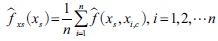where x_s refers to a predictor variable of interest, and x_i,c the other predictor variables.

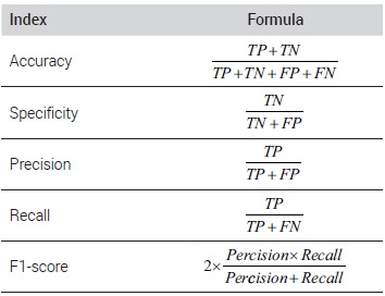
Note 2. The performance evaluation indexes used in this study are described below.

References

Kim, H.N. and Lim, M.Y., 2015. “The Study of Fuel Poverty of the Elderly Households in South Korea”, The Korean Association For Environmental Sociology, 19(2): 133-164.
김하나·임미영, 2015. “사회· 경제적 요인의 에너지 빈곤 영향 분 석: 노인포함가구를 중심으로”, 「환경사회학연구 ECO」, 19(2): 133-164.
Kim, H.K., 2015. “Actual Situation and Policy Implications of Energy Poverty”, Korea Institute for Health and Social Affairs: Sejong.
김현경, 2015. “에너지 빈곤의 실태와 정책적 함의”, 한국보건사회연구원: 세종.
Oh, S.M. and Jin, S.H., 2021. “Path Analysis of Energy Consumption and Poverty Factors of Low-income Households in Seoul”, The Korean Journal of Local Government Studies, 24(4): 29-56.
오수미·진상현, 2021. “서울시 저소득 가구의 에너지 소비 및 빈곤 특성에 관한 경로 분석”, 「지방정부연구」, 24(4): 29-56. [ https://doi.org/10.20484/klog.24.4.2 ]
Lee, H.J., 2019. “Understanding Energy Poverty: Its Definition and Measurement”, Health and Welfare Policy Forum, (273): 6-15.
이현주, 2019. “에너지 빈곤을 어떻게 이해할 것인가: 에너지 빈곤의 정의와 측정”, 「보건복지포럼」, (273): 6-15.
Jin, S.H., Park, E.C., and Hwang, I.C., 2010. “A Study on Definition of Energy Poverty and Estimation of Policy Target”, The Korea Association for Policy Studies, 19(2): 161-182.
진상현·박은철·황인창, 2010. “에너지빈곤의 개념 및 정책대상 추정에 관한 연구”, 「한국정책학회보」, 19(2): 161-182.
Abbas, K., Li, S., Xu, D., Baz, K., and Rakhmetova, A., 2020. “Do Socioeconomic Factors Determine Household Multidimensional Energy Poverty? Empirical Evidence from South Asia”, Energy Policy, 146: 111754. [https://doi.org/10.1016/j.enpol.2020.111754]
Aguilar, M.J., Ramos-Real, F.J., and Ramírez-Díaz, A.J., 2019. “Improving Indicators for Comparing Energy Poverty in the Canary Islands and Spain”, Energies, 12(11): 2135. [https://doi.org/10.3390/en12112135]
Ajay, S., Jatin, R., Rushikesh, P., and Swati, G., 2019. “Poverty Prediction Using Machine Learning”, International Journal of Computer Sciences and Engineering, 7(3): 946-949. [https://doi.org/10.26438/ijcse/v7i3.946949]
Boardman, B., 1991. Fuel Poverty: from Cold Homes to Affordable Warmth, London: Belhaven Press.
Bosch, J., Palència, L., Malmusi, D., Marí-Dell’Olmo, M., and Borrell, C., 2019. “The Impact of Fuel Poverty upon Self-reported Health Status among the Low-income Population in Europe”, Housing Studies, 34(9): 1377-1403. [https://doi.org/10.1080/02673037.2019.1577954]
Boser, B.E., Guyon, I.M., and Vapnik, V.N., 1992. “Atraining Algorithm for Optimal Margin Classifiers”, Proceedings of the Annual Conference on Computational Learning Theory, 144-152. [https://doi.org/10.1145/130385.130401]
Bouzarovski, S. and Petrova, S., 2015. “A Global Perspective on Domestic Energy Deprivation: Overcoming the Energy Poverty–fuel Poverty Binary”, Energy Research and Social Science, 10: 31-40. [https://doi.org/10.1016/j.erss.2015.06.007]
Breiman, L., 1996. “Bagging Predictors”, Machine Learning, 24(2): 123-140. [https://doi.org/10.1007/BF00058655]
Breiman, L., 2001. “Random Forests”, Machine Learning, 45(1): 5-32. [https://doi.org/10.1023/A:1010933404324]
Breiman, L., Friedman, J., Stone, C.J., and Olshen, R.A., 1984. Classification and Regression Trees, Boca Raton: CRC press.
Chalfin, A., Danieli, O., Hillis, A., Jelveh, Z., Luca, M., Ludwig, J., and Mullainathan, S., 2016. “Productivity and Selection of Human Capital with Machine Learning”, American Economic Review, 106(5): 124-27. [https://doi.org/10.1257/aer.p20161029]
Chen, T. and Guestrin, C., 2016. “Xgboost: A Scalable Tree Boosting System”, Proceedings of the 22nd ACM SIGKDD International Conference on Knowledge Discovery and Data Mining, 785-794. [https://doi.org/10.1145/2939672.2939785]
City of Liverpool, 2007. Fuel Poverty and Warm Homes: A Strategy for Liverpool Annual Report. Liverpool.
Crentsil, A.O., Asuman, D., and Fenny, A.P., 2019. “Assessing the Determinants and Drivers of Multidimensional Energy Poverty in Ghana”, Energy Policy, 133: 110884. [https://doi.org/10.1016/j.enpol.2019.110884]
Dubois, U., 2012. “From Targeting to Implementation: The Role of Identification of Fuel Poor Households”, Energy Policy, 49: 107-115. [https://doi.org/10.1016/j.enpol.2011.11.087]
Friedman, J.H., 2001. “Greedy Function Approximation: A Gradient Boosting Machine”, Annals of Statistics, 1189-1232. [https://doi.org/10.1214/aos/1013203451]
Géron, A., 2019. Hands-on Machine Learning with Scikit-Learn, Keras, and TensorFlow: Concepts, Tools, and Techniques to Build Intelligent Systems, Sebastopol: O’Reilly Media.
Greenwell, B.M., 2017. “pdp: An R Package for Constructing Partial Dependence Plots”, The R Journal, 9(1): 421-436. [https://doi.org/10.32614/RJ-2017-016]
Healy, J.D. and Clinch, J.P., 2004. “Quantifying the Severity of Fuel Poverty, Its Relationship with Poor Housing and Reasons for Non-investment in Energy-saving Measures in Ireland”, Energy Policy, 32(2): 207-220. [https://doi.org/10.1016/S0301-4215(02)00265-3]
Hills, J., 2011. Fuel Poverty: The Problem and Its Measurement. Interim Report of the Fuel Poverty Review. Centre for Analysis of Social Exclusion, LSE.
Hills, J., 2012. Getting the Measure of Fuel Poverty: Final Report of the Fuel Poverty Review. Centre for Analysis of Social Exclusion, LSE.
Kaikaew, K., van den Beukel, J.C., Neggers, S.J., Themmen, A.P., Visser, J.A., and Grefhorst, A., 2018. “Sex Difference in Cold Perception and Shivering Onset upon Gradual Cold Exposure”, Journal of Thermal Biology, 77: 137-144. [https://doi.org/10.1016/j.jtherbio.2018.08.016]
Kleinberg, J., Ludwig, J., Mullainathan, S., and Obermeyer, Z., 2015. “Prediction Policy Problems”, American Economic Review, 105(5): 491-95. [https://doi.org/10.1257/aer.p20151023]
Kousis, I., Laskari, M., Ntouros, V., Assimakopoulos, M. N., and Romanowicz, J., 2020. “An Analysis of the Determining Factors of Fuel Poverty among Students Living in the Private-rented Sector in Europe and Its Impact on Their Well-being”, Energy Sources, Part B: Economics, Planning, and Policy, 15(2): 113-135. [https://doi.org/10.1080/15567249.2020.1773579]
Lacroix, E. and Chaton, C., 2015. “Fuel Poverty as a Major Determinant of Perceived Health: the Case of France”, Public Health, 129(5): 517-524. [https://doi.org/10.1016/j.puhe.2015.02.007]
Legendre, B. and Ricci, O., 2015. “Measuring Fuel Poverty in France: Which Households Are the Most Fuel Vulnerable?”, Energy Economics, 49: 620-628. [https://doi.org/10.1016/j.eneco.2015.01.022]
Liaw, A. and Wiener, M., 2002. “Classification and Regression by Random Forest”, R News, 2(3): 18-22.
Masuma, A., 2013. Modelling the Likelihood of Being Fuel Poor, UK: Department of Energy and Climate Change.
Maxim, A., Mihai, C., Apostoaie, C.M., and Maxim, A., 2017. “Energy Poverty in Southern and Eastern Europe: Peculiar Regional Issues”, European Journal of Sustainable Development, 6(1): 247-247. [https://doi.org/10.14207/ejsd.2017.v6n1p247]
McCulloch, W.S. and Pitts, W., 1943. “A Logical Calculus of the Ideas Immanent in Nervous Activity”, The Bulletin of Mathematical Biophysics, 5(4): 115-133. [https://doi.org/10.1007/BF02478259]
Meyer, S., Laurence, H., Bart, D., Middlemiss, L., and Maréchal, K., 2018. “Capturing the Multifaceted Nature of Energy Poverty: Lessons from Belgium”, Energy Research and Social Science, 40: 273-283. [https://doi.org/10.1016/j.erss.2018.01.017]
Molnar, C., 2020. Interpretable Machine Learning: A Guide for Making Black Box Models Explainable. Lulu Press.
Moore, R., 2012. “Definitions of Fuel Poverty: Implications for Policy”, Energy Policy, 49: 19-26. [https://doi.org/10.1016/j.enpol.2012.01.057]
Palmer, G., MacInnes, T., and Kenway, P., 2008. Cold and Poor: An Analysis of the Link between Fuel Poverty and Low Income. Report New Policy Institute.
Price, C.W., Brazier, K., and Wang, W., 2012. “Objective and Subjective Measures of Fuel Poverty”, Energy Policy, 49: 33-39. [https://doi.org/10.1016/j.enpol.2011.11.095]
Romero, J.C., Linares, P., and López, X., 2018. “The Policy Implications of Energy Poverty Indicators”, Energy Policy, 115: 98-108. [https://doi.org/10.1016/j.enpol.2017.12.054]
Rosenblatt, F., 1958. “The Perceptron: A Probabilistic Model for Information Storage and Organization in the Brain”, Psychological Review, 65(6): 386. [https://doi.org/10.1037/h0042519]
Rumelhart, D.E., Hinton, G.E., and Williams, R.J., 1986. “Learning Representations by Back-propagating Errors”, Nature, 323(6088): 533-536. [https://doi.org/10.1038/323533a0]
Sandri, M. and Zuccolotto, P., 2010. “Analysis and Correction of Bias in Total Decrease in Node Impurity Measures for Tree-based Algorithms”, Statistics and Computing, 20(4): 393-407. [https://doi.org/10.1007/s11222-009-9132-0]
Sharma, A. and Kumar, H., 2019. “Seasonal Variation on Electricity Consumption of Academic Building-A Case Study”, Journal of Thermal Energy System, 2(2): 1-6.
Snell, C., Bevan, M., and Thomson, H., 2015. “Justice, Fuel Poverty and Disabled People in England”, Energy Research and Social Science, 10: 123-132. [https://doi.org/10.1016/j.erss.2015.07.012]
Sovacool, B.K., 2015. “Fuel Poverty, Affordability, and Energy Justice in England: Policy Insights from the Warm Front Program”, Energy, 93: 361-371. [https://doi.org/10.1016/j.energy.2015.09.016]
Tod, A.M., Lusambili, A., Homer, C., Abbott, J., Cooke, J.M., Stocks, A.J., and McDaid, K.A., 2012. “Understanding Factors Influencing Vulnerable Older People Keeping Warm and Well in Winter: A Qualitative Study Using Social Marketing Techniques”, BMJ Open, 2(4). [https://doi.org/10.1136/bmjopen-2012-000922]
Verme, P., 2020. Which Model for Poverty Predictions?. Global Labor Organization.